2.1 Temperature REMD simulation of a small peptide
Files for this tutorial (tutorial-2.1.tar.gz)
Contents
- 2.1.1 Setup
- 2.1.2. minimization and pre-equilibration
- 2.1.3 Equilibration
- 2.1.4. Production
- 2.1.5 Analysis of REMD simulation
- 2.1.5.1. Calculate the acceptance ratio of each replica
- 2.1.5.2. Plot time courses of replica indices and temperatures
- 2.1.5.3. Plot time courses of potential energy of each replica
- 2.1.5.4. Sort coordinates in DCD trajectory files by parameters
- 2.1.5.5. Principal Component Analysis (PCA)
- 2.1.5.5.3 eigmat_analysis
- References
In this tutorial, we illustrate how to perform a replica-exchange molecular dynamics (REMD) simulations with GENESIS. REMD method is one of the enhanced conformational sampling methods used for systems with rugged free energy landscape. In temperature REMD (T-REMD), we prepare multiple copies (replicas) of the original system with different temperature assigned. The temperature can be exchanged between each pair of replicas during the simulation. The random walk in temperature space results in the simulation surmounting energy barriers and sampling much wider conformational space of target molecule [1].
In GENESIS, not only T-REMD, but also pressure REMD, surface-tension REMD (γ-REMD) [2], replica-exchange umbrella sampling (REUS), and their multi-dimensional version are available.
REMD simulation in GENESIS requires an MPI environment. At least one MPI processor must be assigned to one replica.
Please note that it may take more than 12 hours to finish all simulations in this tutorial.
2.1.1 Setup
All files for this tutorial are packed into an archive just below the title of this tutorial. The input files to be used are already prepared in the 1_setup directory. In this directory, we have wbox.pdb (coordinate file), wbox.psf (CHARMM structure file), par_all36_prot.prm (CHARMM parameter file), top_all36_prot.rtf (CHARMM topology file), and toppar_water_ions.str (CHARMM topology and parameter file for TIP3P water and ions).
# make a new directory to do this tutorial
$ mkdir tutorial-2.1
$ cd tutorial-2.1

# copy and decompress the downloaded file
$ cp ~/Download/tutorial-2.1.tar.gz ./
$ tar -xvzf tutorial-2.1.tar.gz
$ cd tutorial-2.1
$ ls
1_setup  2_minimize_pre-equi  3_equilibrate  4_production  5_analysis

# check the initial PDB structure
$ ls ./1_setup
build               top_all36_prot.rtf     wbox.log  wbox.psf
par_all36_prot.prm  toppar_water_ions.str  wbox.pdb
$ vmd ./1_setup/wbox.pdb
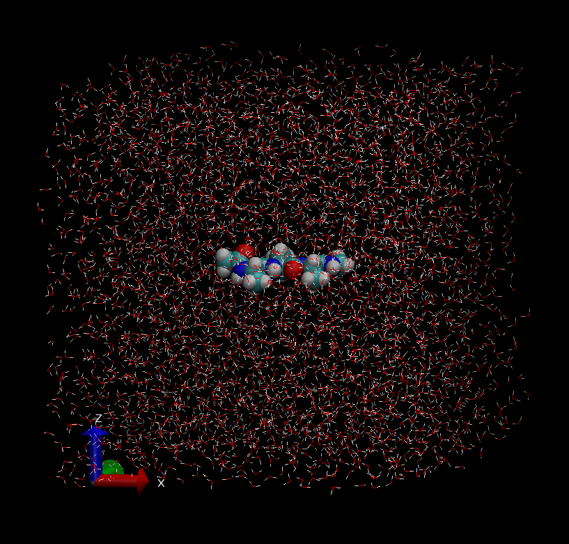
The system is composed of one alanine tripeptide and 3,939 TIP3P waters. In the initial structure, and the initial box size is (x, y, z) = (50.2Å, 50.2Å, 50.2Å). In the initial structure, the peptide forms a fully extended conformation with the backbone dihedral angle (φ, ψ) = (180°, 180°). This model was created using CHARMM and VMD (see “./1_setup/build/” if you are interested in the modeling).
2.1.2. minimization and pre-equilibration
In the directories “2_minimize_pre-equi”, “3_equilibrate” and “4_production”, there are not only control files “*.inp“, but also batch job scripts file “*.sh“. For example, in the directory “2_minimize_pre-equi”, there are 4 control files and 1 job script file as follows:
# change directory
$ cd 2_minimize_pre-equi
$ ls
step2.sh step2.1.inp step2.2.inp step2.3.inp step2.4.inp
The bathc job script file “step2.sh" is as follows:
$ more ./step2.sh
#! /bin/bash -f
#
#$ -S /bin/bash
#$ -cwd
#$ -V
#$ -pe ompi 16
#$ -q  nogpu.q
#$ -N  minim_pre-equi

export OMP_NUM_THREADS=2
bindir=/home/user/genesis/bin

mpirun -machinefile ${TMP}/machines -np 8 -npernode 8 ${bindir}/spdyn step2.1.inp > step2.1.log
mpirun -machinefile ${TMP}/machines -np 8 -npernode 8 ${bindir}/spdyn step2.2.inp > step2.2.log
mpirun -machinefile ${TMP}/machines -np 8 -npernode 8 ${bindir}/spdyn step2.3.inp > step2.3.log
mpirun -machinefile ${TMP}/machines -np 8 -npernode 8 ${bindir}/spdyn step2.4.inp > step2.4.log
Please change the green-colored parts according to the PC cluster system you use. For the details on the batch job script, please see the Usage page.
You can run this job script as follows:
# perform minimization and pre-equilibration with SPDYN by using 8 MPI processors
$ qsub step2.sh
We explain the details about the control files “*.inp” in the following subsections.
2.1.2.1. Minimization
Because the initial structures often contain non-physical steric clashes or non-equilibrium geometries, we should relax the system before the REMD simulation by minimizing the potential energy of the system. atdyn and spdyn support the steepest descent algorithm for minimization, which moves atoms proportionally to their negative gradients of the potential energy. Here we use spdyn, but you can also use atdyn instead of spdyn:
The control file “step2.1.inp” consists of several sections such as [INPUT], [OUTPUT], [ENERGY] and so on, where we specify the control parameters for the simulation.
[INPUT]
topfile = ../1_setup/top_all36_prot.rtf     # topology file for protein
parfile = ../1_setup/par_all36_prot.prm     # parameter file for protein
strfile = ../1_setup/toppar_water_ions.str  # topology and parameter file for water and ions
psffile = ../1_setup/wbox.psf    # protein structure file
pdbfile = ../1_setup/wbox.pdb    # PDB file
reffile = ../1_setup/wbox.pdb    # PDB file for restraints

[OUTPUT]
dcdfile = step2.1.dcd            # dcd trajectory file
rstfile = step2.1.rst            # restart file

[ENERGY]
forcefield       = CHARMM	       # CHARMM force field
electrostatic    = PME           # particle Mesh Ewald Method
switchdist       = 10.0          # switch distance
cutoffdist       = 12.0          # cutoff distance
pairlistdist     = 13.5          # pair-list distance
vdw_force_switch = YES           # force switch option for van der Waals
contact_check    = YES           # avoid calculation failure due to atomic crash

[MINIMIZE]
method           = SD            # steepest descent method
nsteps           = 2000          # number of minimization steps
eneout_period    = 100           # energy output period
crdout_period    = 100           # coordinate output period
rstout_period    = 2000          # restart output period
nbupdate_period  = 10            # nonbond update period

[BOUNDARY]
type             = PBC           # periodic boundary condition
box_size_x       = 50.2          # box size (x) in [PBC]
box_size_y       = 50.2          # box size (y) in [PBC]
box_size_z       = 50.2          # box size (z) in [PBC]

[SELECTION]
group1 = sid:PROA and heavy      # select heavy atoms of alanine tripeptide

[RESTRAINTS]
nfunctions      = 1              # Number of restraint functions
function1       = POSI           # positional restraint
direction1      = all            # direction
constants1      = 1.0            # force constant of a restraint function
select_index1   = 1              # Index of a atom group for the restraint
In [INPUT] section, input files for the minimization are specified. topfile (topology file), parfile (parameter file), psffile (structure file) and pdbfile (initial structure) are required when you use CHARMM force field parameter set. If an optional input, crdfile (charmm coordinate file), is specified, coordinates in the crdfile are used as the initial coordinates prior to those in pdbfile.
If you use AMBER force field parameter set, you specify file names of prmtopfile (amber prmtop format file) and ambcrdfile (rst7 ascii format file) instead of topfile, prmfile, strfile, crdfile and psffile (see this page).
In [OUTPUT] section, output files are specified. spdyn does not create any output file unless you explicitly specify the files. Here, rstfile (restart file) is used for the restart of the simulation, and dcdfile (trajectory file) for output of the trajectory. Bear in mind that the files you are going to create must not be already present in the directory you specify.
In [ENERGY] section, you set the keywords related to the energy and force evaluation. Here the particle mesh Ewald (PME) method is selected to compute electrostatic interactions, usually combined with the periodic boundary condition (PBC) stated in [BOUNDARY] section. contact_check option is avaialble in minimization step only, and this option is used to avoid calculation failure due to bad steric clash often included in your initial structures.
[MINIMIZE] section turns on minimization engine of spdyn. Here we specify 2000 steps of the steepest descent algorithm (SD).
In [BOUNDARY] section, the boundary conditions and the simulation box size are set. Here you use the periodic boundary conditions (PBC). box_size_x, box_size_y, box_size_z specify the box dimensions of the system. These values are necessary in the first minimization step.
In [RESTRAINTS] section, positional restraints are applied to the atom group “group1” which consists of heavy atoms of the peptide. This atom group is defined in the [SELECTION] section. The restraints are imposed with respect to the reference coordinates given by reffile in [INPUT] section.
2.1.2.2. Equilibration of the system at 300 K
After the minimization, we equilibrate the system under the condition of 300 K by a 10 ps MD simulation.
The control file (step2.2.inp) used for this step is as follows:
[INPUT]
topfile = ../1_setup/top_all36_prot.rtf    # topology file for protein
parfile = ../1_setup/par_all36_prot.prm    # parameter file for protein
strfile = ../1_setup/toppar_water_ions.str # topology and parameter file for water and ions
psffile = ../1_setup/wbox.psf     # protein structure file
pdbfile = ../1_setup/wbox.pdb     # PDB file
reffile = ../1_setup/wbox.pdb     # reference file
rstfile = step2.1.rst             # restart file

[OUTPUT]
dcdfile = step2.2.dcd        # dcd trajectory file
rstfile = step2.2.rst        # restart file

[ENERGY]
forcefield       = CHARMM    # use CHARMM force field
electrostatic    = PME       # use particle Mesh Ewald Method
switchdist       = 10.0      # switch distance
cutoffdist       = 12.0      # force cutoff distance
pairlistdist     = 13.5      # pair-list distance
vdw_force_switch = YES       # force switch option for van der Waals
pme_nspline      = 4         # order of B-spline in [PME]
pme_max_spacing  = 1.0       # max grid spacing

[DYNAMICS]
integrator      = LEAP       # leapfrog Verlet integrator
nsteps          = 5000       # number of MD steps
timestep        = 0.002      # time interval of MD step, unit [ps]
eneout_period   =   10       # energy output period
crdout_period   =  100       # coordinate output period
rstout_period   = 5000       # restart output period
nbupdate_period =   10       # nonbond pairlist update period

[ENSEMBLE]
ensemble        = NVT        # use NVT ensemble
temperature     = 300.00     # intial and terget temperature, unit [K]
tpcontrol       = LANGEVIN   # use Langevin thermostat

[CONSTRAINTS]
rigid_bond      = YES        # use SHAKE/SETTLE constraints

[BOUNDARY]
type = PBC                   # periodic boundary condition

[SELECTION]
group1 = sid:PROA and heavy  # select heavy atoms of alanine tripeptide

[RESTRAINTS]
nfunctions      = 1          # Number of restraint functions
function1       = POSI       # positional restraint
direction1      = all        # direction
constants1      = 1.0        # force constant of a restraint function
select_index1   = 1          # Index of a atom group for the restraint
[CONSTRAINTS] section specifies constraints during a simulation. “rigid_bond” is a keyword to use SHAKE algorithm for the peptide molecule. For water molecules, a faster algorithm (SETTLE algorithm) is automatically applied if rigid_bond = YES. In [BOUNDARY] section, we do not specify the box dimensions, because the values are read from the rstfile. In [ENSEMBLE] section, we choose Langevin thermostat. In this simulation run, we use NVT ensemble, and the temperature is set to 300.00 K.
2.1.2.3. Relaxation of the simulation box
After the system reached the desired temperature 300.00 K, we relax the simulation box by 10 ps MD simulation.
The control file (step2.3.inp) is as follows:
[INPUT]
topfile = ../1_setup/top_all36_prot.rtf    # topology file for protein
parfile = ../1_setup/par_all36_prot.prm    # parameter file for protein
strfile = ../1_setup/toppar_water_ions.str # topology and parameter file for water and ions
psffile = ../1_setup/wbox.psf     # protein structure file
pdbfile = ../1_setup/wbox.pdb     # PDB file
rstfile = step2.2.rst             # restart file

[OUTPUT]
dcdfile = step2.3.dcd             # DCD trajectory file
rstfile = step2.3.rst             # restart file

[DYNAMICS]
integrator      = LEAP       # leapfrog Verlet integrator
nsteps          = 5000       # number of MD steps
timestep        = 0.002      # time interval of MD step, unit [ps]
eneout_period   =   10       # energy output period
crdout_period   =  100       # coordinate output period
rstout_period   = 5000       # restart output period
nbupdate_period = 10         # nonbond pairlist update period

[ENERGY]
forcefield       = CHARMM    # use CHARMM force field
electrostatic    = PME       # use particle Mesh Ewald Method
switchdist       = 10.0      # switch distance
cutoffdist       = 12.0      # force cutoff distance
pairlistdist     = 13.5      # pair-list distance
vdw_force_switch = YES       # force switch option for van der Waals
pme_nspline      = 4         # order of B-spline in [PME]
pme_max_spacing  = 1.0       # max grid spacing

[CONSTRAINTS]
rigid_bond = YES             # use SHAKE/SETTLE constraints

[ENSEMBLE]
ensemble    = NPT            # use NPT ensemble
temperature = 300.00         # temperature, unit [K]
pressure    = 1.0            # pressure, unit [atm]
tpcontrol   = LANGEVIN       # use Langevin thermostat/barostat
isotropy    = ISO            # isotropic pressure scaling

[BOUNDARY]
type = PBC                   # periodic boundary condition

[SELECTION]
group1 = sid:PROA and heavy  # select heavy atoms of dialanine

[RESTRAINTS]
nfunctions      = 1          # Number of restraint functions
function1       = POSI       # positional restraint
direction1      = all        # direction
constants1      = 1.0        # force constant of a restraint function
select_index1   = 1          # Index of a atom group for the restraint
In this pre-equilibration run, we use NPT ensemble, and isotropy is set to ‘ISO‘ so that the X, Y and Z dimensions are coupled together.
2.1.2.4. Equilibration with no positional restraints
Finally we run an additional 10-ps pre-equilibration simulation, in which we relax all atom positions including the peptide atoms with no positional restraints. The control file (step2.4.inp) is as follows:
[INPUT]
topfile = ../1_setup/top_all36_prot.rtf    # topology file for protein
parfile = ../1_setup/par_all36_prot.prm    # parameter file for protein
strfile = ../1_setup/toppar_water_ions.str # topology and parameter file for water and ions
psffile = ../1_setup/wbox.psf     # protein structure file
pdbfile = ../1_setup/wbox.pdb     # PDB file
rstfile = step2.3.rst             # restart file

[OUTPUT]
dcdfile = step2.4.dcd             # DCD trajectory file
rstfile = step2.4.rst             # restart file

[DYNAMICS]
integrator      =  LEAP    # leapfrog Verlet integrator
nsteps          =  5000    # number of MD steps
timestep        = 0.002    # time interval of MD step, unit [ps]
eneout_period   =    10    # energy output period
crdout_period   =   100    # coordinate output period
rstout_period   =  5000    # restart output period
nbupdate_period =    10    # nonbond pairlist update period

[ENERGY]
forcefield       = CHARMM  # use CHARMM force field
electrostatic    = PME     # use particle Mesh Ewald Method
switchdist       = 10.0    # switch distance
cutoffdist       = 12.0    # force cutoff distance
pairlistdist     = 13.5    # pair-list distance
vdw_force_switch = YES     # force switch option for van der Waals
pme_nspline      = 4       # order of B-spline in [PME]
pme_max_spacing  = 1.0     # max grid spacing

[CONSTRAINTS]
rigid_bond = YES           # use SHAKE/SETTLE constraints

[ENSEMBLE]
ensemble    = NPT          # use NPT ensemble
temperature = 300.00       # temperature, unit [K]
pressure    = 1.0          # pressure, unit [atm]
tpcontrol   = LANGEVIN     # use LANGEVIN thermostat/barostat
isotropy    = ISO          # isotropic pressure scaling

[BOUNDARY]
type = PBC                 # periodic boundary condition
2.1.3 Equilibration
Before starting T-REMD simulation, we must determine the number of replicas and the temperatures of replicas. These temperatures have to be chosen carefully, because they greatly affect the results of T-REMD simulations and probabilities of the replica exchanges. If the difference of temperatures between adjacent replicas is small, the exchange probability is high, but the number of replicas needed for such simulation is also large. Therefore, we need to find the optimal temperature intervals to perform efficient REMD simulations, but it may be troublesome [3].
We recommend using the web server REMD Temperature generator [4]. This tool automatically generates the number of replicas and their temperatures according to the information we input. We show the example of the input for the T-REMD simulation of the solvated trialanine system:
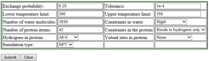
Replica exchange probabilities are often set to 0.2 – 0.3, and here we set the replica exchange probability to 0.25. The lower and upper temperature limits are set to 300 K and 350 K, respectively. Since we use SHAKE and SETTLE algorithms in the simulation, “constraints in the protein” is set to “Bonds to hydrogen only”, and “Constraints in water” to “rigid”. We use all-atom model, so we select “All H” for the parameter of “Hydrogens in proteins”. The numbers of protein atoms and the water molecules are input according to the numbers in "../1_setup/wbox.pdb“. We can count the number of the water molecules in the system as follows:
# count the number of TIP3P water molecules
$ grep "TIP3" ../1_setup/wbox.pdb | wc -l | awk '{print $1 / 3}'
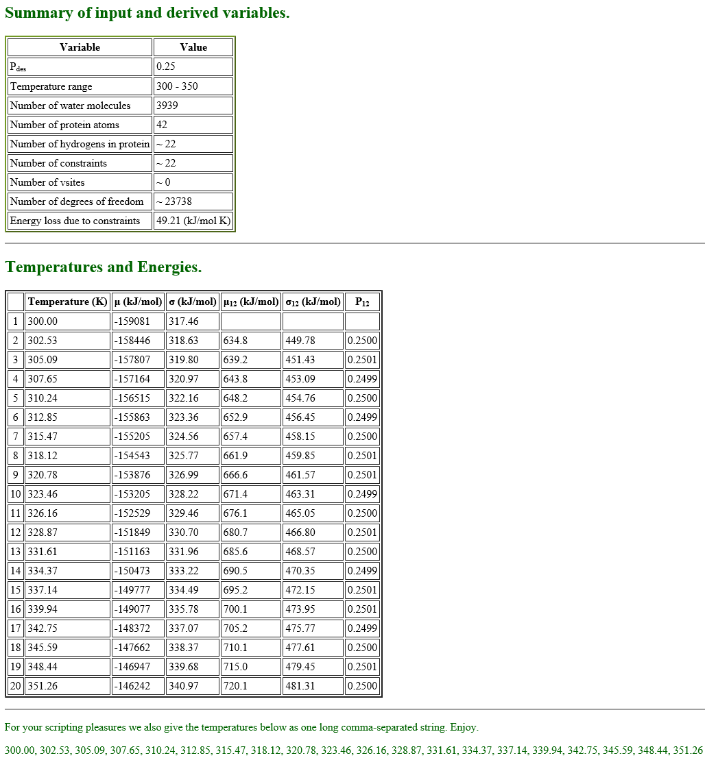
When we fill in all the parameters and submit them, the server generates the summary, temperatures and energies of 20 replicas in a few seconds as follows.
In the table shown above, there is the parameter “Simulation type“. We can select either “NPT” or “NVT” for the parameter, but, when we select “NVT“, the server returns an error message. Thus we choose “NPT” here, even though we use NVT ensemble in our T-REMD simulation.
 Using these generated temperature parameters, we start our T-REMD simulation. First, each replica must be equilibrated at the selected temperature just like conventional MD simulations. The following command performs a 10-ps NVT MD simulations. Here we use 160 (= 8 x 20) MPI processors for the REMD simulations, because we use 8 MPI processors for each replica, and we need 20 replicas.
# change to the equilibration directory
$ cd ../3_equilibrate
$ ls
step3.inp step3.sh

$ more ./step3.sh
#! /bin/bash -f
#$ -S /bin/bash
#$ -cwd
#$ -V
#$ -pe ompi 160
#$ -q  nogpu.q
#$ -N  remd_eq

export OMP_NUM_THREADS=1
bindir=/home/user/genesis/bin
mpirun -machinefile ${TMP}/machines -np 160 -npernode 16 ${bindir}/spdyn step3.inp > step3.log

# perform equilibration at each temperature with SPDYN by submitting batch job script $ qsub ./step3.sh
Let’s view the control file ‘step3.inp‘ (see also this page for more details about the input files for T-REMD simulations).
[INPUT]
topfile = ../1_setup/top_all36_prot.rtf        # topology file
parfile = ../1_setup/par_all36_prot.prm        # parameter file
strfile = ../1_setup/toppar_water_ions.str     # stream file
psffile = ../1_setup/wbox.psf                  # protein structure file
pdbfile = ../1_setup/wbox.pdb                  # PDB file
rstfile = ../2_minimize_pre-equi/step2.4.rst   # restart file

[OUTPUT]
dcdfile  = step3_rep{}.dcd      # DCD trajectory file
rstfile  = step3_rep{}.rst      # restart file
remfile  = step3_rep{}.rem      # replica exchange ID file
logfile  = step3_rep{}.log      # log file of each replica

[ENERGY]
forcefield       = CHARMM       # CHARMM force field
electrostatic    = PME          # Particle Mesh Ewald method
switchdist       = 10.0         # switch distance
cutoffdist       = 12.0         # cutoff distance
pairlistdist     = 13.5         # pair-list distance
vdw_force_switch = YES          # force switch option for van der Waals
pme_nspline      = 4            # order of B-spline in [PME]
pme_max_spacing  = 1.0          # max grid spacing

[DYNAMICS]
integrator       =  LEAP        # leapfrog Verlet integrator
nsteps           =  5000        # number of MD steps
timestep         = 0.002        # timestep (ps)
eneout_period    =   500        # energy output period
crdout_period    =   500        # coordinates output period
rstout_period    =  5000        # restart output period
nbupdate_period  =    10        # nonbond update period

[CONSTRAINTS]
rigid_bond       = YES          # use SHAKE/SETTLE algorithms

[ENSEMBLE]
ensemble         = NVT          # NVT ensemble
tpcontrol        = LANGEVIN     # thermostat and barostat
temperature      = 300.00       # initial and target temperature (K)

[BOUNDARY]
type             = PBC          # periodic boundary condition

[REMD]
dimension        = 1            # number of parameter types
exchange_period  = 0            # NO exchange for equilibration

type1            = temperature  # T-REMD
nreplica1        = 20           # number of replicas
parameters1      = 300.00 302.53 305.09 307.65 310.24 \
                   312.85 315.47 318.12 320.78 323.46 \
                   326.16 328.87 331.61 334.37 337.14 \
                   339.94 342.75 345.59 348.44 351.26
In [INPUT] section, we specify step2.4.rst file as the restart file of the simulation run. In the REMD simulation, the 20 (equal to the number of replicas specified nreplica in [REMD] section explained below) copies are automatically made from this restart file.
In [OUTPUT] section, in addition to dcdfile and rstfile names, we give also logfile and remfile. If we perform REMD simulations, file names of logfile and remfile are also required. logfile gives a log file of MD simulation for each replica. remfile gives replica exchange parameter. In this section, “{}” returns a replica index number from 1 to 20.
When we want to run REMD simulations, we add [REMD] section in the control file. In [REMD] section, the number of dimensions is set to dimension = 1, and the type of the exchanged variable is set to type1 = temperature for T-REMD simulation. The number of replicas is set to nreplica1 = 20, and we assign the replica temperatures to the variable parameter1. If exchange_period = 0, then no exchanges occur during the run, and so we set exchange_period to 0 for equilibration of all replicas.
In [ENSEMBLE] section, we change NPT ensemble to NVT ensemble. Though we can perform REMD simulations both in NVT and NPT ensemble with GENESIS, we recommend performing T-REMD simulations in NVT ensemble, because in a temperature exceeding the water boiling point, the system may be disrupted.
Other parameters in [INPUT], [ENERGY], [ENSEMBLE], [BOUNDARY] and [CONSTRAINTS] sections are not changed from the previous runs (“step2.4.inp“).
2.1.4. Production
After the equilibration, we perform the production run of T-REMD. The following commands perform a 5-ns simulation in NVT ensemble:
# change to the production directory
$ cd ../4_production
$ ls
step4.inp step4.sh

# perform REMD production run with SPDYN by submitting batch job script $ qsub ./step4.sh
Let’s look at the control file “step4.inp“.
[INPUT]
topfile = ../1_setup/top_all36_prot.rtf        # topology file
parfile = ../1_setup/par_all36_prot.prm        # parameter file
strfile = ../1_setup/toppar_water_ions.str     # stream file
psffile = ../1_setup/wbox.psf                  # protein structure file
pdbfile = ../1_setup/wbox.pdb                  # PDB file
rstfile = ../3_equilibrate/step3_rep{}.rst     # restart file

[OUTPUT]
dcdfile  = step4_rep{}.dcd      # DCD trajectory file
rstfile  = step4_rep{}.rst      # restart file
remfile  = step4_rep{}.rem      # replica exchange ID file
logfile  = step4_rep{}.log      # log file of each replica

[ENERGY]
forcefield       = CHARMM       # CHARMM force field
electrostatic    = PME          # Particle Mesh Ewald method
switchdist       = 10.0         # switch distance
cutoffdist       = 12.0         # cutoff distance
pairlistdist     = 13.5         # pair-list distance
vdw_force_switch = YES          # force switch option for van der Waals
pme_nspline      = 4            # order of B-spline in [PME]
pme_max_spacing  = 1.0          # max grid spacing

[DYNAMICS]
integrator       = LEAP         # leapfrog Verlet integrator
nsteps           = 2500000      # number of MD steps
timestep         = 0.002        # timestep (ps)
eneout_period    =   500        # energy output period
crdout_period    =   500        # coordinates output period
rstout_period    =  5000        # restart output period
nbupdate_period  =    10        # nonbond update period

[CONSTRAINTS]
rigid_bond       = YES          # use SHAKE/SETTLE constraints

[ENSEMBLE]
ensemble         = NVT          # NPT ensemble
tpcontrol        = LANGEVIN     # thermostat and barostat
temperature      = 300.00       # initial and target temperature (K)

[BOUNDARY]
type             = PBC          # periodic boundary condition

[REMD]
dimension        = 1            # number of parameter types
exchange_period  = 2500         # attempt exchange every 5 ps

type1            = temperature  # T-REMD
nreplica1        = 20           # number of replicas
parameters1      = 300.00 302.53 305.09 307.65 310.24 \
                   312.85 315.47 318.12 320.78 323.46 \
                   326.16 328.87 331.61 334.37 337.14 \
                   339.94 342.75 345.59 348.44 351.26
In [INPUT] section, rstfile points to the output files from the equilibration. “{}” returns a series of the 20 input files.
In [REMD] section, the period between replica exchanges is specified by exchange_period = 2500. Then replica exchange attempts occurs every 2500 steps, that is, every 5 ps. The other parameters in [REMD] section should not be changed from those in the input files of your previous runs.
In the log output of the REMD simulation (“step4.log”), we can see the information about replica-exchange attempts at every exchange_period steps.
REMD> Step:    2497500   Dimension:    1   ExchangePattern:    2
  Replica      ExchangeTrial             AcceptanceRatio      Before       After
        1         16 >    17   A         230 /       500     339.940     342.750
        2         19 >    18   R         209 /       500     348.440     348.440
        3         12 >    13   A         194 /       500     328.870     331.610
        4          4 >     5   R         194 /       500     307.650     307.650
        5          6 >     7   R         196 /       500     312.850     312.850
        6         10 >    11   A         222 /       500     323.460     326.160
        7          5 >     4   R         194 /       500     310.240     310.240
        8          7 >     6   R         196 /       500     315.470     315.470
        9         14 >    15   R         199 /       500     334.370     334.370
       10         11 >    10   A         222 /       500     326.160     323.460
       11         13 >    12   A         194 /       500     331.610     328.870
       12          3 >     2   A         192 /       500     305.090     302.530
       13         20 >     0   N           0 /         0     351.260     351.260
       14          8 >     9   R         185 /       500     318.120     318.120
       15         17 >    16   A         230 /       500     342.750     339.940
       16         18 >    19   R         209 /       500     345.590     345.590
       17          1 >     0   N           0 /         0     300.000     300.000
       18         15 >    14   R         199 /       500     337.140     337.140
       19          2 >     3   A         192 /       500     302.530     305.090
       20          9 >     8   R         185 /       500     320.780     320.780

Parameter    :    342.750   348.440   331.610   307.650   312.850   326.160   310.240   315.470   334.370   323.460   328.870   302.530   351.260   318.120   339.940   345.590   300.000   337.140   305.090   320.780
RepIDtoParmID:         17        19        13         4         6        11         5         7        14        10        12         2        20         8        16        18         1        15         3         9
ParmIDtoRepID:         17        12        19         4         7         5         8        14        20        10         6        11         3         9        18        15         1        16         2        13

REMD> Step:    2500000   Dimension:    1   ExchangePattern:    1
  Replica      ExchangeTrial             AcceptanceRatio      Before       After
        1         17 >    18   A         210 /       500     342.750     345.590
        2         19 >    20   R         212 /       500     348.440     348.440
        3         13 >    14   A         215 /       500     331.610     334.370
        4          4 >     3   R         197 /       500     307.650     307.650
        5          6 >     5   R         213 /       500     312.850     312.850
        6         11 >    12   A         212 /       500     326.160     328.870
        7          5 >     6   R         213 /       500     310.240     310.240
        8          7 >     8   R         178 /       500     315.470     315.470
        9         14 >    13   A         215 /       500     334.370     331.610
       10         10 >     9   R         205 /       500     323.460     323.460
       11         12 >    11   A         212 /       500     328.870     326.160
       12          2 >     1   R         194 /       500     302.530     302.530
       13         20 >    19   R         212 /       500     351.260     351.260
       14          8 >     7   R         178 /       500     318.120     318.120
       15         16 >    15   A         224 /       500     339.940     337.140
       16         18 >    17   A         210 /       500     345.590     342.750
       17          1 >     2   R         194 /       500     300.000     300.000
       18         15 >    16   A         224 /       500     337.140     339.940
       19          3 >     4   R         197 /       500     305.090     305.090
       20          9 >    10   R         205 /       500     320.780     320.780

Parameter    :    345.590   348.440   334.370   307.650   312.850   328.870   310.240   315.470   331.610   323.460   326.160   302.530   351.260   318.120   337.140   342.750   300.000   339.940   305.090   320.780
RepIDtoParmID:         18        19        14         4         6        12         5         7        13        10        11         2        20         8        15        17         1        16         3         9
ParmIDtoRepID:         17        12        19         4         7         5         8        14        20        10        11         6         9         3        15        18        16         1         2        13
In this log file, we should pay attention to the AcceptanceRatio values. If those values are extremely low, you should review the parameters of your simulation. In this example, we want to achieve the probability of exchanges at a level of 0.25. For instance, the AcceptanceRatio of replica 1 in ExchangePattern: 2 is 230 / 500, so 0.46. We will calculate the average AcceptanceRatio values in the next part of this tutorial.
In this table, ‘A‘ and ‘R‘ mean that the accepted and rejected exchange trials, respectively. ‘N‘ denotes the replicas which cannot be exchanged at this attempt, because there is no pair for replica IDs 1 and 20 in the ExchangePattern: 2. The last two columns show replica temperatures before and after the exchange trials, respectively.
Lines in purple summarize the locations and parameters after replica exchanges. The Parameter line gives the temperature of each replica in T-REMD simulation. The RepIDtoParmID line stands for the permutation function that converts Replica ID to Parameter ID. For example, in the 1st column, 18 is written, which means that the temperature of Replica 1 is set to 345.59 K. The ParmIDtoRepID line also represents the permutation function that converts Parameter ID to Replica ID. For example, in the 6th column, 5 is written, which means that Parameter 6 (corresponding to the replica temperature, 313.00 K) is located in Replica 5.
2.1.5 Analysis of REMD simulation
In this section, we explain how to analyze T-REMD trajectories. All analyses are carried out in the 5_analysis directory. Here we use gnuplot and various linux commands such as grep, tee, tail, sed, and awk, and also utilize a pipe (|) to combine the commands. For your convenience, all the commands have been included in the “*.sh” scripts.
# change directory
$ cd ../5_analysis
$ ls
1_calc_ratio  2_plot_index  3_plot_potential  4_sort_dcd  5_PCA
2.1.5.1. Calculate the acceptance ratio of each replica
As we mentioned in the previous section, acceptance ratio of replica exchange is one of the important factors that determine the efficiency of REMD simulations. The acceptance ratio is displayed in a standard log output “step4.log“, and we examine the data from the last step. Here, we show an example how to examine the data. Note that the acceptance ratio of replica “A” to “B” is identical to “B” to “A”, and thus we calculate only “A” to “B”. For this calculation, you can use the script “calc_ratio.sh“.
# change directory
$ cd 1_calc_ratio

# make the file executable and use it
$ chmod u+x calc_ratio.sh
$ ./calc_ratio.sh

1 > 2 0.388
3 > 4 0.394
5 > 6 0.426
7 > 8 0.356
9 > 10 0.41
11 > 12 0.424
13 > 14 0.43
15 > 16 0.448
17 > 18 0.42
19 > 20 0.424
The file “calc_ratio.sh” contains the following commands:
# get acceptance ratios between adjacent parameter IDs
$ grep "  1 >     2" ../../4_production/step4.log | tail -1  > acceptance_ratio.dat
$ grep "  3 >     4" ../../4_production/step4.log | tail -1 >> acceptance_ratio.dat
$ grep "  5 >     6" ../../4_production/step4.log | tail -1 >> acceptance_ratio.dat
....
$ grep " 19 >    20" ../../4_production/step4.log | tail -1 >> acceptance_ratio.dat

# calculate the ratios
$ awk '{print $2,$3,$4,$6/$8}' acceptance_ratio.dat
In the case illustrated above, the obtained ratio (~ 0.4) is larger than the expected ratio 0.25. The two ratios are so different possibly because of the use of a very small peptide.
2.1.5.2. Plot time courses of replica indices and temperatures
To examine the random walks of each replica in temperature space, we analyze time course of the replica indices. We need to plot the values of the “ParmIDtoRepID” lines from step4.log for a chosen starting replica temperature, for example 300 K (first column), versus time. Using following commands, we can get replica IDs in each snapshot.
# change directory
$ cd ../2_plot_indes

# make the file executable and use it
$ chmod u+x plot_index.sh
$ ./plot_index.sh
The file “plot_index.sh” contains the following commands:
# get replica IDs in each snapshot
$ grep "ParmIDtoRepID:" ../../4_production/step4.log | sed 's/ParmIDtoRepID:/ /' > T-REMD_parmID-repID.dat
Using following gnuplot commands, we can plot the replica IDs in each snapshot.
# plot replica IDs in each snapshot
$ gnuplot
gnuplot> set yrange [0:21]
gnuplot> set mxtics
gnuplot> set mytics
gnuplot> set xlabel "Time (ns)"
gnuplot> set ylabel "Replica ID"
gnuplot> plot "T-REMD_parmID-repID.dat" using ($0*0.005):1 with points pt 5 ps 0.5 lc rgb "cyan" title "300.00 K"
gnuplot> plot "T-REMD_parmID-repID.dat" using ($0*0.005):10 with points pt 7 ps 0.5 lc rgb "green" title "323.46 K"
gnuplot> plot "T-REMD_parmID-repID.dat" using ($0*0.005):20 with points pt 9 ps 0.5 lc rgb "red" title "351.26 K"

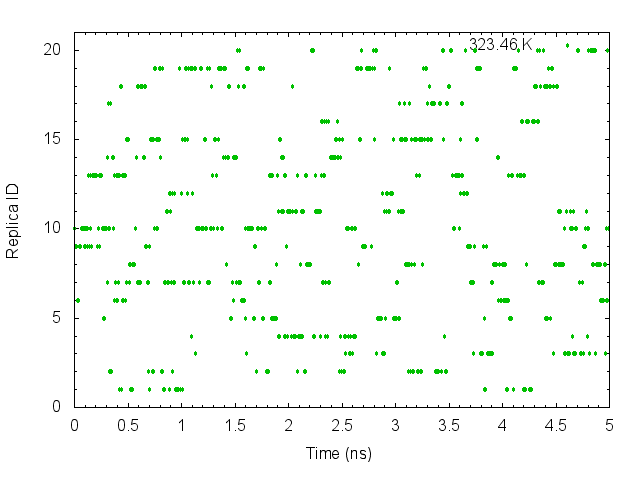
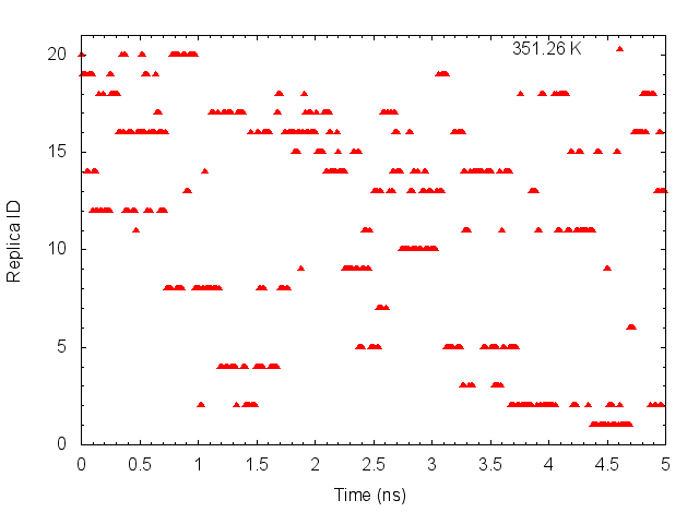
These graphs indicate that the temperatures (parameterIDs) visit randomly each replica, and thus random walks in the temperature spaces are successfully realized.
We also plot time courses of temperatures in one replica. We need to plot one column in the “Parameter :” lines in step4.log versus time. Using following commands. we can get replica temperatures in each snapshot.
# make the file executable and use it
$ chmod u+x plot_temperature.sh
$ ./plot_temperature.sh
The file “plot_temperature.sh” contains the following commands:
# get replica temperatures in each snapshot
$ grep "Parameter    :" ../../4_production/step4.log | sed 's/Parameter    :/ /' > T-REMD_repID-temperatrue.dat
Using following gnuplot commands, we can plot the replica IDs in each snapshot.
# plot replica temperatures in each snapshot
$ gnuplot
gnuplot> set mxtics
gnuplot> set mytics
gnuplot> set xlabel "Time (ns)"
gnuplot> set ylabel "Temperature (K)"
gnuplot> plot "T-REMD_repID-Temperature.dat" using ($0*0.005):1  with lines lc rgb "cyan" title "repID=1 "
gnuplot> replot "T-REMD_repID-Temperature.dat" using ($0*0.005):10 with lines lc rgb "green" title "repID=10"
gnuplot> replot "T-REMD_repID-Temperature.dat" using ($0*0.005):20 with lines lc rgb "red" title "repID=20"
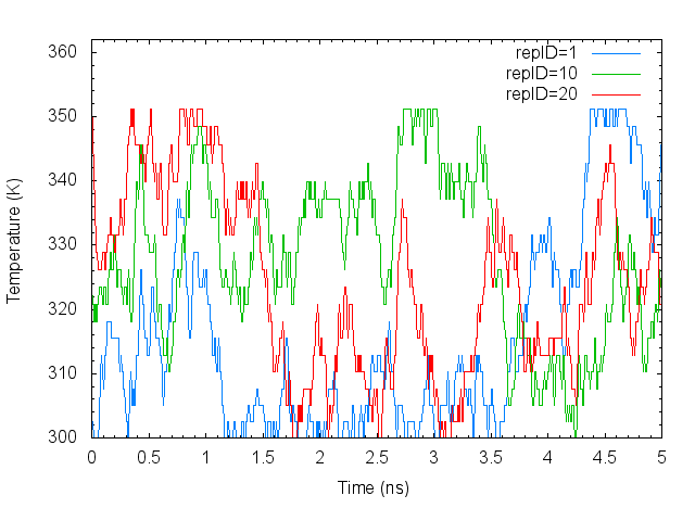
The temperatures of each replica during the simulation are distributed in all temperatures assigned. It means that correct annealing of the system is realized.
2.1.5.3. Plot time courses of potential energy of each replica
The aim of usingT-REMD method is to surmount high energy barriers and to move another potential minimum. Therefore, in replicas whose temperature is high, the potential energies of the replicas must be high depending on their replica temperatures. The potential energy is written in the logfiles ‘step4_rep{}.log‘, and using these logfiles, we can check the potential energy of each replica as follows:
# change directory
$ cd ../3_plot_potential

# make the file executable and use it
$ chmod u+x plot_potential.sh
$ ./plot_potential.sh
The file “plot_potential.sh” contains the following commands:
# get the potential energy of each replica
$ grep "INFO:" ../../4_production/step4_rep1.log  | tail -n +2 | awk '{print $5} > potential_energy_rep1.dat
$ grep "INFO:" ../../4_production/step4_rep10.log | tail -n +2 | awk '{print $5} > potential_energy_rep10.dat
$ grep "INFO:" ../../4_production/step4_rep20.log | tail -n +2 | awk '{print $5} > potential_energy_rep20.dat
Using following gnuplot commands, we can plot the potential energies in each snapshot.
# plot potential energies
$ gnuplot
gnuplot> set xlabel "Time (ns)"
gnuplot> set ylabel "Potential energy (kcal/mol)"
gnuplot> plot "potential_energy_rep1.dat" using ($0*0.001):1 with lines lc rgb "cyan" title "repID=1"
gnuplot> replot "potential_energy_rep10.dat" using ($0*0.001):1 with lines lc rgb "green" title "repID=10"
gnuplot> replot "potential_energy_rep20.dat" using ($0*0.001):1 with lines lc rgb "red" title "repID=20"
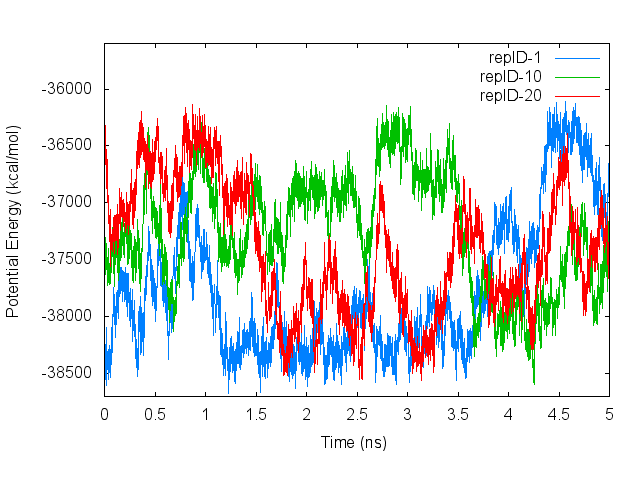
Let’s compare the plots containing changes in the replica temperatures and changes in the potential energies. We can see that the potential energies increase and decrease depending on the replica temperatures.
2.1.5.4. Sort coordinates in DCD trajectory files by parameters
The T-REMD output files contain DCD trajectories prepared for each replicaIDs. Therefore the temperatures in each trajectory change in time. To sort the frames of trajectories by parameterIDs (or by the same temperatures), we can use remd_convert of the GENESIS analysis tool set. Sorting is done based on the information written in remfiles generated from the REMD simulation.
# change directory
$ cd ../4_sort_dcd

# sort coordinates by parameters
$ /home/user/genesis/bin/remd_convert step5.remd_convert.inp | tee step5.remd_convert.log
Let’s view the “step5.remd_convert.inp“.
[INPUT]
psffile = ../../1_setup/wbox.psf                # protein structure file
reffile = ../../1_setup/wbox.pdb                # PDB file
dcdfile = ../../4_production/step4_rep{}.dcd    # DCD trajectory file
remfile = ../../4_production/step4_rep{}.rem    # replica exchange ID file

[OUTPUT]
pdbfile = trialanine.pdb                        # output PDB file
trjfile = remd_paramID{}_trialanine.dcd         # output trajectory file

[SELECTION]
group1  = atomno:1-42                           # trialanine atoms
group2  = resno:2 and (an:N or an:CA or an:C or an:O)  # main-chain atoms of residue 2

[FITTING]
fitting_method = TR+ROT
fitting_atom   = 2
mass_weight    = YES

[OPTION]
check_only     = NO
convert_type   = PARAMETER
convert_ids    = 1             # (empty = all)
dcd_md_period  = 500           # coordinates output period
trjout_format  = DCD           # (PDB/DCD)
trjout_type    = COOR+BOX      # (COOR/COOR+BOX)
trjout_atom    = 1             # output atom selection
pbc_correct    = NO            # (wrap molecules)
In the [INPUT] section, the psffile (contains system information) and reffile (atom coordinate file) are required. In addition to the two files, we specify dcdfile (DCD trajectory file) and remfile (replica information file) obtained in the REMD production run. In the [OPTION] section, convert_type = PARAMETER is used to sort coordinates by replica parameters. For dcd_md_period, we set the same value as the crdout_period in the REMD control file. By selecting only peptide atoms by “trjout_atom“, we can extract the trajectory of peptide only at each replica temperature. We set convert_ids = 1 in order to obtain the peptide structures at 300.00 K (parameterID = 1).
When you use the mass-weighted fitting in crd_convert and remd_convert (mass_weight = YES in the [FITTING] section), you must specify psffile (for CHARMM) or prmtopfile (for AMBER) in the [INPUT] section. This is because, in these programs, atom masses are read from the structure files.
After sorting the coordinates, we can examine conformations ot the peptide at ambient temperatures, for example, by following commands:
# check the sorted dcd file for ParameterID 1 (300.00 K)
$ vmd ../1_setup/wbox.pdb -dcd ./remd_trj_paramID1.dcd

# examine Ramachandran diagram
$ /home/user/genesis/bin/trj_analysis step5.trj_rama.inp | tee step5.trj_rama.log
The one of the simplest ways to study a protein structure is to examine the Ramachandran diagram. You can examine the two dihedral angles Φ and ψ using trj_analysis included in GENESIS analysis tools. In the input file “step5.trj_rama.inp“, we specify the number of atoms included in each snapshot by “trj_natom = 42” in [TRAJECTORY] section. This is because the trajectory file “remd_trj_paramID1.dcd” contains the coordinates of the peptide atoms only.
[INPUT]
psffile = ../1_setup/wbox.psf                  # protein structure file
reffile = ../1_setup/wbox.pdb                  # PDB file

[OUTPUT]
torfile = rama_trj_paramID1.tor                # torsion angle file

[TRAJECTORY]
trjfile1      = remd_paramID1_trialanine.dcd   # output trajectory file
md_step1      = 2500000                        # number of MD steps
mdout_period1 = 500                            # MD output period
ana_period1   = 500                            # analysis period

trj_format    = DCD                            # (PDB/DCD)
trj_type      = COOR+BOX                       # (COOR/COOR+BOX)
trj_natom     = 42                             # the number of atoms included in each snapshot

[OPTION]
check_only = NO
torsion1   = PROA:1:ALA:C  \
             PROA:2:ALA:N  \
             PROA:2:ALA:CA \
             PROA:2:ALA:C        # PHI angle
torsion2   = PROA:2:ALA:N  \
             PROA:2:ALA:CA \
             PROA:2:ALA:C  \
             PROA:3:ALA:N        # PSI angle
We can plot the Ramachandran diagram using following gnuplot commands:
$ gnuplot
gnuplot> set xrange [-180 : 180]
gnuplot> set yrange [-180 : 180]
gnuplot> set xtics 60
gnuplot> set ytics 60
gnuplot> set mxtics
gnuplot> set mytics
gnuplot> set xlabel "PHI (deg)"
gnuplot> set ylabel "PSI (deg)"
gnuplot> set size square
gnuplot> plot "rama_trj_paramID1.tor" using 2:3 with points pt 7 lt 3 notitle
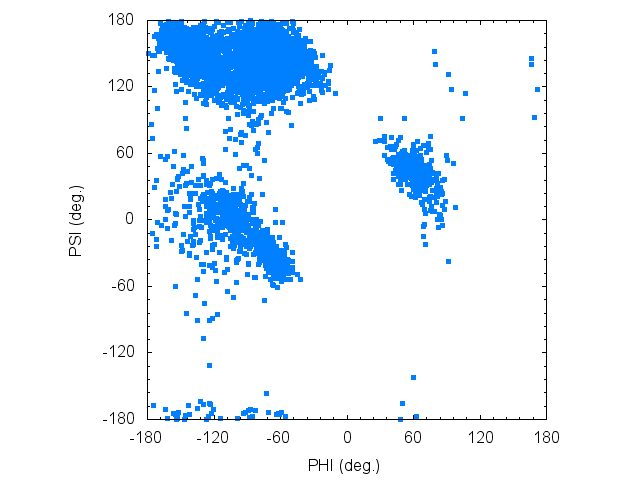
In the Ramachandran plot, one can see both an extended structure like β-strand, and a bent structures like α-helix.
2.1.5.5. Principal Component Analysis (PCA)
To study the conformation of the short peptide, it might be enough to examine the Ramachandran plot. However, in general, the proteins of interest have many residues. One of the efficient ways to study the protein conformation sampled with REMD simulations is to perform principal component analysis (PCA). Here, we illustrate how to perform PCA using GENESIS (see also the tutorial page of PCA).
To perform PCA using GENESIS, we need 4 analysis programs shown below:
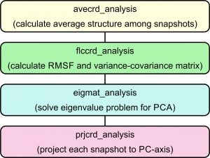
Here, we explain the 4 programs in the order shown in the flowchart.
# change directory
$ cd ../5_PCA
$ ls
step5.avecrd_analysis.inp step5.eigmat_analysis.inp step5.flccrd_analysis.inp step5.prjcrd_analysis.inp step5.pcaana.sh
2.1.5.5.1 avecrd_analysis
This program calculates the average structure during the MD simulation. To do this, we use the following command:
# calculate the averaged conformation during the MD simulation
$ /home/user/genesis/bin/avecrd_analysis step5.avecrd_analysis.inp | tee step5.avecrd_analysis.log
Let’s look at the input file “step5.avecrd_analysis.inp”
[INPUT]
psffile = ../../1_setup/wbox.psf         # protein structure file
reffile = ../../1_setup/wbox.pdb         # PDB file

[OUTPUT]
rmsfile     = remd_paramID1_avecrd.rms   # file for RMSD output
pdb_avefile = remd_paramID1_avecrd.pdb   # PDB file (Averaged coordinates of analysis atoms)
pdb_aftfile = remd_paramID1_fitcrd.pdb   # PDB file (Averaged coordinates of fitting atoms)

[TRAJECTORY]
trjfile1      = ../4_sort_dcd/remd_paramID1_trialanine.dcd
md_step1      = 2500000                        # number of MD steps
mdout_period1 = 500                            # MD output period
ana_period1   = 500                            # analysis period

trj_format = DCD                               # (PDB/DCD)
trj_type   = COOR+BOX                          # (COOR/COOR+BOX)
trj_natom  = 42

[SELECTION]
group1 = atomno:1-42 and heavy                 # the peptide non-hydrogen atoms
group2 = resno:2 and (an:N or an:CA or an:C or an:O) # main-chain atoms of residue 2

[FITTING]
fitting_method = TR+ROT                  # method
fitting_atom   = 2                       # atom group used for fitting
mass_weight    = YES                     # mass-weight is applied

[OPTION]
check_only     = NO                       # (YES/NO)
num_iterations = 3                        # number of iterations
analysis_atom  = 1                        # analysis target atom group
The [INPUT] and [TRAJECTORY] sections are identical with those in “step5.remd_convert.inp“. In this program, fitting is done to calculate the average structure. In [FITTING] section, fitting method and atom group used for fitting are specified. The number of iterations of fitting is given by num_iterations in [OPTION] section. Atom group used for averaging is specified by “analysis_atom“. Output file names are shown in [OUTPUT] section. The average coordinates of analyzed atoms and of fitted atoms are written in pdb_avefile and pdb_aftfile, respectively.
2.1.5.5.2 flccrd_analysis
Next, we calculate the root mean squared fluctuations of the peptide atoms and the variance-covariance matrix. To do this, we use the following command:
$ /home/user/genesis/bin/flccrd_analysis step5.flccrd_analysis.inp | tee step5.flccrd_analysis.log
Let’s look at the input file “step5.flccrd_analysis.inp”
[INPUT]
psffile = ../../1_setup/wbox.psf        # protein structure file
reffile = ../../1_setup/wbox.pdb        # PDB file
pdb_avefile = remd_paramID1_avecrd.pdb  # PDB file (Averaged coordinates of analysis atoms)
pdb_aftfile = remd_paramID1_fitcrd.pdb  # PDB file (Averaged coordinates of fitting atoms)

[OUTPUT]
rmsfile     = remd_paramID1_rmsf.dat  # file for RMSF output
pcafile     = remd_paramID1_pca.dat   # variance-covariance matrix for all selected atoms
vcvfile     = remd_paramID1_vcv.dat   # variance-covariance matrix file for only CA atoms in selection
crsfile     = remd_paramID1_crs.dat   # cross-correlation matrix file for only CA atoms in selection

[TRAJECTORY]
trjfile1      = ../4_sort_dcd/remd_paramID1_trialanine.dcd
md_step1      = 2500000                        # number of MD steps
mdout_period1 = 500                            # MD output period
ana_period1   = 500                            # analysis period

trj_format = DCD                               # (PDB/DCD)
trj_type   = COOR+BOX                          # (COOR/COOR+BOX)
trj_natom  = 42

[SELECTION]
group1 = atomno:1-42 and heavy                       # the peptide non-hydrogen atoms
group2 = resno:2 and (an:N or an:CA or an:C or an:O) # main-chain atoms of residue 2

[FITTING]
fitting_method = TR+ROT                 # method
fitting_atom   = 2                      # atom group used for fitting
mass_weight    = YES                    # mass-weight is applied

[OPTION]
check_only    = NO                      # (YES/NO)
vcv_matrix    = global                  # (GLOBAL/LOCAL)
analysis_atom = 1                       # analysis target atom group
For this analysis program, we require not only psffile and pdbfile, but also pdb_avefile and pdb_aftfile generated by the program avecrd_analysis. In [OPTION] section, if vcv_matrix = global, RMSF values and variance-covariance matrix are calculated for the analysis target atoms specified by analysis_atom. If vcv_matrix = local, RMSF values and variance-covariance matrix are calculated for the fitting target atoms specified by fitting_atom. The variance-covariance matrix calculated using all target atoms are saved in pcafile. This file name is specifed in [OUTPUT] section.
2.1.5.5.3 eigmat_analysis
To diagonalize the variance-covariance matrix obtained using flccrd_analysis, we use the program eigmat_analysis:
$ /home/user/genesis/bin/eigmat_analysis step5.eigmat_analysis.inp | tee step5.eigmat_analysis.log
Let’s look at the input file “step5.eigmat_analysis.inp”
[INPUT]
pcafile = remd_paramID1_pca.dat  # variance-covariance matrix for all selected atoms

[OUTPUT]
valfile = remd_paramID1_val.dat  # output of eigenvalues
vecfile = remd_paramID1_vec.dat  # output of eigenvectors
cntfile = remd_paramID1_cnt.dat  # output of contribution of each mode
This program diagonalizes the variance-covariance matrix, so only pcafile is required as an input. In [OUTPUT] section, we specify the 3 ouput file names, valfile, vecfile, and cntfile. In these files, eigenvalue, eigenvector and contribution of each PC mode are saved, respectively.
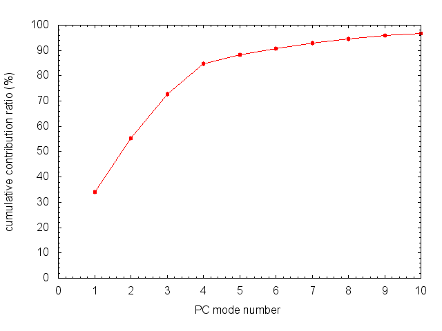
To plot the cumulative contribution ratio, we use the following gnuplot commands:
$ gnuplot
gnuplot> set xlabel "PC mode number"
gnuplot> set ylabel "cumulative contribution ratio (%)"
gnuplot> set xrange [0:10]
gnuplot> set yrange [0:100]
gnuplot> set xtics 1
gnuplot> set ytics 10
gnuplot> set mxtics
gnuplot> set mytics
gnuplot> plot "remd_paramID1_cnt.dat" using 1:4 with lp pointtype 7 notitle
2.1.5.5.4 prjcrd_analysis
Since we obtained the eigenvalues and the eigenvectors of the variance-covariance matrix, we can finally project each snapshot from the trajectory onto the calculated PC axes. We use the following command:
$ /home/user/genesis/bin/prjcrd_analysis step5.prjcrd_analysis.inp | tee step5.prjcrd_analysis.log
Let’s look at the input file “step5.prjcrd_analysis.inp”
[INPUT]
psffile     = ../../1_setup/wbox.psf    # protein structure file
reffile     = ../../1_setup/wbox.pdb    # PDB file
pdb_avefile = remd_paramID1_avecrd.pdb  # PDB file (Averaged coordinates of analysis atoms)
pdb_aftfile = remd_paramID1_fitcrd.pdb  # PDB file (Averaged coordinates of fitting atoms)
valfile     = remd_paramID1_val.dat     # output of eigenvalues
vecfile     = remd_paramID1_vec.dat     # output of eigenvectors

[OUTPUT]
prjfile     = remd_paramID1_prjcrd.dat  # output of principal components of each snapshot

[TRAJECTORY]
trjfile1      = ../4_sort_dcd/remd_paramID1_trialanine.dcd
md_step1      = 2500000                         # number of MD steps
mdout_period1 = 500                             # MD output period
ana_period1   = 500                             # analysis period

trj_format = DCD                                # (PDB/DCD)
trj_type   = COOR+BOX                           # (COOR/COOR+BOX)
trj_natom  = 42

[SELECTION]
group1 = atomno:1-42 and heavy          # the peptide non-hydrogen atoms
group2 = resno:2 and (an:N or an:CA or an:C or an:O) # main-chain atoms of residue 2

[FITTING]
fitting_method = TR+ROT                 # method
fitting_atom   = 2                      # atom group used for fitting
mass_weight    = YES                    # mass-weight is applied

[OPTION]
check_only    = NO                      # (YES/NO)
vcv_matrix    = global                  # (GLOBAL/LOCAL)
num_pca       = 4                       # number of principal components
analysis_atom = 1                       # analysis target atom group
Using the prjfile, we can get the conformational distribution by plotting (PC2, PC3) with gnuplot:
$ gnuplot
gnuplot> set xlabel "PC2"
gnuplot> set ylabel "PC3"
gnuplot> set mxtics
gnuplot> set mytics
gnuplot> plot "remd_paramID1_prjcrd.dat" using 3:4 with points ps 0.5 pt 7 notitle
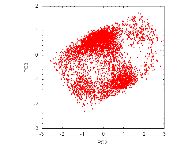 There are three clusters in the PC2-PC3 plot ((PC2, PC3) = (0.0, 0.6), (0.8, 1.0), (-1.0, -1.4)).
References
- Yuji Sugita, Yuko Okamoto, “Replica-exchange molecular dynamics method for protein folidng.” Chem. Phys. Lett., 314, 141-151 (1999)
- Takaharu Mori, Jaewoon Jung, and Yuji Sugita, “Surface-tension replica-exchange molecular dynamics method for enhanced sampling of biological membrane systems”, J. Chem. Theory Comput., 9, 5629-5640 (2013).
- Y. Sanbonmatsu and A. E. Garcia, “Structure of Met-Enkephalin in Explicit Aqueous Solution Using Replica Exchange Molecular Dynamics.” Proteins, 46, 225-234 (2002).
- A. Patriksson & D. van der Spoel, “A temperature predictor for parallel tempering simulations.” Phys. Chem. Chem. Phys., 10, 2073-2077 (2008).
Written by Daisuke Matsuoka@RIKEN Theoretical molecular science laboratory
July, 28, 2016