2.2 Replica-exchange umbrella sampling
Files for this tutorial (tutorial-2.2.tar.gz)
Contents
Conformational sampling is one of the most important issues in the computational biophysics field. Because complex biomolecules have many local-minimum energy states, conventional MD simulations often get trapped there, resulting in that unreliable free energy profile is obtained. Umbrella sampling method has been widely used to calculate free energy profile. In this method, several different restraint potentials are applied to the system along the reaction coordinates, and histograms of the reaction coordinates are analyzed by using a reweighting technique such as WHAM to obtain the potential of mean force . In 2000, Sugita et al. proposed the replica-exchange umbrella sampling method (REUS , which is also called Hamiltonian REMD or Window exchange umbrella sampling ), in which the restraint potentials are exchanged between replicas to enhance conformational sampling. In this tutorial, we demonstrate a REUS simulation of a small peptide using GENESIS. We show typical analyses for REUS trajectories, and discuss the folding mechanism of the peptide based on the free energy profile. Please note that it may take more than 12 hours to finish all simulations in this tutorial.
2.2.1 Setup
Tutorial files are available from the link just below the title of this turotial. Let us see the contents in the downloaded file by the following commands. The initial PDB structure (wbox.pdb) is contained in the 1_setup directory. In this tutorial, we use the same target system (alanine tripeptide in water) with 2.1 REMD tutorial. So, we do not explain the system setup again. For details, please see “2.1.1 Setup” in the REMD tutorial.
# make a new directory to do this tutorial
$ mkdir tutorial-2.2
$ cd tutorial-2.2

# copy and decompress the downloaded file
$ cp ~/Download/tutorial-2.2.tar.gz ./
$ tar -xzf tutorial-2.2.tar.gz
$ cd tutorial-2.2
$ ls
1_setup  2_minimize_pre-equi  3_equilibrate  4_production  5_analysis
2.2.2 Minimization and pre-equilibration
First of all, we carry out energy minimization for the initial PDB structure (./1_setup/wbox.pdb) and perform short MD simulations to prepare an equilibrated initial structure for the subsequent REUS simulation. Here, we perform 2000 steps energy minimization and 30 ps MD simulations step by step. The followings are sample commands. If you are using a cluster machine and need a batch script to run commands, please make it by yourself. This section is also same with “2.1.2 Minimization and pre-equilibration” in 2.1 REMD tutorial. For detailed explanation about this protocol, see that section. At the end of Step2.4, we obtain the restart file step2.4.rst, which will be used in the next.
# change directory
$ cd 2_minimize_pre-equi

# perform 2000steps energy minimization and 3 x 10ps equilibration runs
$ mpirun -np 8 /home/user/genesis/bin/spdyn step2.1.inp > log2.1
$ mpirun -np 8 /home/user/genesis/bin/spdyn step2.2.inp > log2.2
$ mpirun -np 8 /home/user/genesis/bin/spdyn step2.3.inp > log2.3
$ mpirun -np 8 /home/user/genesis/bin/spdyn step2.4.inp > log2.4
2.2.3 Equilibration
Final goal of this tutorial is to calculate the free energy profile (or potential of mean force) as a function of the end-to-end distance of the alanine tripeptide. We are going to use 14 replicas in the REUS simulation. Since each replica has an individual restraint potential, we should shortly equilibrate the structure (step2.4.rst) using 14 different restraints. In Step3, we perform these equilibrations. Let us see the control file:
# change directory
$ cd ../3_equilibrate

# check the control file (only important sections are shown below)
$ less step3.inp
[INPUT]
topfile = ../1_setup/top_all36_prot.rtf       # topology file
parfile = ../1_setup/par_all36_prot.prm       # parameter file
strfile = ../1_setup/toppar_water_ions.str    # stream file
psffile = ../1_setup/wbox.psf                 # protein structure file
pdbfile = ../1_setup/wbox.pdb                 # PDB file
rstfile = ../2_minimize_pre-equi/step2.4.rst  # restart file

[OUTPUT]
logfile = step3_rep{}.log    # log file of each replica
dcdfile = step3_rep{}.dcd    # DCD trajectory file
rstfile = step3_rep{}.rst    # restart file

[REMD]
dimension        = 1
exchange_period  = 0
iseed            = 3141592
type1            = RESTRAINT
nreplica1        = 14
cyclic_params1   = NO
rest_function1   = 1

[SELECTION]
group1     = an:OY  and resno:1  # restraint group 1
group2     = an:HNT and resno:3  # restraint group 2

[RESTRAINTS]
nfunctions = 1
function1  = DIST
constant1  = 1.2 1.2 1.2 1.2 1.2 1.2 1.2 1.2 1.2 1.2 1.2 1.2 1.2 1.2
reference1 = 1.80 2.72 3.64 4.56 5.48 6.40 7.32 8.24 9.16 10.08 11.00 11.92 12.84 13.76
select_index1 = 1 2
This control file is almost same with the subsequent production run of the REUS simulation, but we specify exchange_period = 0 in the [REMD] section, which means that parameter exchange does not occur. In the [REMD], [SELECTION], and [RESTRAINTS] sections, we give REUS parameters. We apply restraints on the distance between N-terminus and C-terminus, where OY atom in Residue 1 and HNT atom in Residue 3 are selected. The target distance is ranging from 1.80 to 13.76Å at the interval of 0.92Å, and the force constant of the restraint potential is set to 1.2 kcal/mol/Å2 for all replicas. Note that 1.80Å nearly corresponds to the hydrogen bond distance, and 13.76Å is a distance when the peptide forms a fully extended conformation.

Index of the restraint function to be used in REUS is specified in rest_function in [REMD] (red character above), and parameters to be exchanged in REUS are specified in constant and reference in [RESTRAINTS]. Note that values in the same column in constant and reference lines are packed into one “parameter set”, and they are exchanged between replicas. For example, if the user specifies “constant1 = 1.2 1.4 1.6” and “reference1 = 1.80 2.72 3.64“, each replica has (1.2, 1.80) or (1.4, 2.72) or (1.6, 3.64).
In the [OUTPUT] section, we can see that there is a bracket “{}” in the filename. The replica number is automatically inserted into this bracket. For example, Replica1 yields step3_rep1.log, step3_rep1.dcd, and step3_rep1.rst.
For other sections such as [ENERGY], [DYNAMICS], [CONSTRAINTS], and [ENSEMBLE], we use typical parameters used in the conventional MD simulations. The simulation is performed in the NVT ensemble at 300K, and Langevin thermostat is used for temperature control. The SHAKE/SETTLE algorithms are applied to the bonds including hydrogen and TIP3P water. We carry out 100ps MD simulation for each replica to equilibrate the system.
Let us execute spdyn by the following command. Sample of the batch script file (run.sh) is also included in the 3_equilibrate directory, which should be modified according to the user’s machine environment. Here, we use 8 MPI processors for one replica, and we need 8 MPI processors x 14 replicas = 112 MPI processors in total.
$ mpirun -np 112 /home/user/genesis/bin/spdyn step3.inp > step3.log
Number of MPI processors in each replica is automatically set to “total MPI processors ÷ number of replicas”. In addition, each replica keeps the rule of hybrid MPI/OpenMP parallelization for single MD simulation.
After the simulation is finished, let us check the peptide conformation of each replica by VMD:
# for Replica 1
$ vmd ../1_setup/wbox.pdb -psf ../1_setup/wbox.psf -dcd step3_rep1.dcd

# for Replica 14
$ vmd ../1_setup/wbox.pdb -psf ../1_setup/wbox.psf -dcd step3_rep14.dcd
We can see that the peptide conformation in Replica1 (short distance restraint) is compact, while it is extended in Replica 14 (long distance restraint), indicating that equilibration with 14 individual restrains was done correctly.
2.2.4 Production run
We carry out the production run of the REUS simulation. Let us see the control file:
# change directory
$ cd ../4_production

# check the control file (only important sections are shown below)
$ less step4.inp
[INPUT]
topfile = ../1_setup/top_all36_prot.rtf     # topology file
parfile = ../1_setup/par_all36_prot.prm     # parameter file
strfile = ../1_setup/toppar_water_ions.str  # stream file
psffile = ../1_setup/wbox.psf               # protein structure file
pdbfile = ../1_setup/wbox.pdb               # PDB file
rstfile = ../3_equilibrate/step3_rep{}.rst  # restart file

[OUTPUT]
logfile = step4_rep{}.log   # log file of each replica
dcdfile = step4_rep{}.dcd   # DCD trajectory file
rstfile = step4_rep{}.rst   # restart file
remfile = step4_rep{}.rem   # parameter index file

[REMD]
dimension        = 1
exchange_period  = 1000
type1            = RESTRAINT
nreplica1        = 14
cyclic_params1   = NO
rest_function1   = 1

[DYNAMICS]
integrator       = LEAP     # Leapfrog Verlet integrator
nsteps           = 2000000  # number of MD steps in REMD
timestep         = 0.002    # timestep (ps)
eneout_period    = 50       # energy output period
crdout_period    = 50       # coordinates output period
rstout_period    = 2000000  # restart output period
nbupdate_period  = 10       # nonbond update period
We specify “exchange_period = 1000” in the [REMD] section to exchange parameters between replicas. Other simulation conditions are same with the previous equilibration. In the [OUTPUT] section, we define remfile, where the parameter index in each replica is output during the simulation. We perform 4 ns REUS simulation for each replica (4 ns x 14 replicas = 56 ns in total). Coordinates are output every 50 steps.
Like the previous equilibration run, we execute spdyn by the following command. Sample of the batch script file (run.sh) is also included in the 4_production directory.
$ mpirun -np 112 /home/user/genesis/bin/spdyn step4.inp > step4.log
In step4.log, information about replica-exchange attempt is output at every exchange_period steps. For example, at 55000 step you can see the following (or similar) information:
REMD> Step:   55000     Dimension:   1     ExchangePattern:   2
  Replica  ExchangeTrial        AcceptanceRatio      Before    After
        1        1 >   0   N          0 /     0           1        1
        2        6 >   7   R          5 /    28           6        6
        3        4 >   5   R          2 /    28           4        4
        4        5 >   4   R          2 /    28           5        5
        5        2 >   3   R          4 /    28           2        2
        6        8 >   9   R          6 /    28           8        8
        7        3 >   2   R          4 /    28           3        3
        8        7 >   6   R          5 /    28           7        7
        9       10 >  11   A          6 /    28          10       11
       10        9 >   8   R          6 /    28           9        9
       11       12 >  13   A          7 /    28          12       13
       12       11 >  10   A          6 /    28          11       10
       13       14 >   0   N          0 /     0          14       14
       14       13 >  12   A          7 /    28          13       12

 Parameter    :   1   6   4   5   2   8   3   7   11   9  13   10   14   12
 RepIDtoParmID:   1   6   4   5   2   8   3   7   11   9  13   10   14   12
 ParmIDtoRepID:   1   5   7   3   4   2   8   6   10  12   9   14   11   13
The red line tells us that Replica 9 had Parameter 10 (k = 1.2, r = 10.08) before 55000 step, and the exchange to Parameter 11 (k = 1.2, r = 11.00) was accepted (A) at 55000 step, and then it has Parameter 11 after 55000 step. The acceptance ratio between the parameter pairs 10 and 11 at 55000 step is 6/28 (=21.4%). The blue line tells us that Replica 3 had Parameter 4 (k = 1.2, r = 4.56), but the exchange to Parameter 5 (k = 1.2, r = 5.48) was rejected (R), and then it has still Parameter 4 after 55000 step. The green lines tell us that Replicas 1 and 13 have Parameter 1 and 14, respectively, but they have no neighboring pairs. Thus, replica exchange was not attempted (N) at this step.
We can see that ExchangePattern is 2 at 55000 step. In the exchange pattern = 2, Parameters 2-3, Parameters 4-5, Parameters 6-7, …, and Parameters 12-13 are defined as the neighboring pairs and exchanged. On the other hand, in the exchange pattern = 1, Parameters 1-2, Parameters 3-4, Parameters 5-6, …, and Parameters 13-14 are defined as the neighboring pairs and exchanged. In the one-dimensional REMD simulation, exchange pattern = 1 and 2 emerge alternatively at every exchange_period.
Purple lines summarize location of replica and parameter indexes. The RepIDtoParmID line stands for the permutation function that converts Replica ID to Parameter ID. For example, in the 2nd column, 6 is written, which means that Replica 2 has Parameter 6. In the 6th column, 8 is written, indicating that Replica 6 has Parameter 8. The ParmIDtoRepID line also stands for the permutation function that converts Parameter ID to Replica ID. For example, in the 6th column, 2 is written, which means that Parameter 6 is located in Replica 2. In the 8th column, 6 is written, indicating that Parameter 8 is located in Replica 6. The Parameter line includes parameter index of each replica. In the case of REUS, this line is same with RepIDtoParmID line (In the temperature REMD simulation, temperature values are shown in the Parameter line).
After the simulation is finished, we obtain trajectory and restart files from each replica.
If you want to restart the REUS simulation, do NOT change the order of the replica parameters in the control file before and after the restart, even if parameter exchange occurred during the simulation.
[RESTRAINTS]
constant1  = 1.2 1.2 1.2 1.2 1.2 1.2 1.2 1.2 1.2 1.2 1.2 1.2 1.2 1.2
reference1 = 1.80 2.72 3.64 4.56 5.48 6.40 7.32 8.24 9.16 10.08 11.00 11.92 12.84 13.76
2.2.5 Analysis
In this section, we explain how to analyze REUS trajectories. All analyses are carried out in the 5_analysis directory. Note that we will use various linux commands such as grep, cut, paste, tail, sed, and awk, and also utilize a pipe (|) to combine the commands. Please, learn their basic usage in advance, if you do not know.
# change directory
$ cd ../5_analysis
$ ls
1_convert_dcd  2_sort_dcd  3_calc_ratio  4_plot_index  5_calc_dist  6_calc_wham
1. Make converted trajectory files for analysis
Because the obtained raw DCD files contain many water molecules, it may take much time to analyze them. In order to save the analysis time, we first remove all water molecules from the trajectory files and create new DCD files by using crd_convert of the GENESIS analysis tool set. In addition, we superimpose the peptide structure of each snapshot onto the initial structure with respect to the backbone atoms. Sample control file for crd_convert is put in the 1_dcd_convert directory:
# change directory
$ cd 1_convert_dcd
$ ls
INP1   INP11  INP13  INP2  INP4  INP6  INP8  run.csh
INP10  INP12  INP14  INP3  INP5  INP7  INP9  script

# remove water and make new DCD files
# this is done for 1 to 14 (./run.csh is available for scripting)
$ /home/user/genesis/bin/crd_convert INP1 > log1
$ /home/user/genesis/bin/crd_convert INP2 > log2
:
$ /home/user/genesis/bin/crd_convert INP14 > log14

# check the converted trajectory file by VMD
$ vmd ./step4_rep1.pdb -dcd ./step4_rep1.dcd
When you use the mass-weighted fitting in crd_convert and remd_convert (mass_weight = YES in the [FITTING] section), you must specify psffile (for CHARMM) or prmtopfile (for AMBER) in the [INPUT] section. This is because, in these programs, atom masses are read from the structure files.
2. Sort coordinates in DCD files by parameters
In the raw DCD files generated from the REUS simulation, coordinates at different conditions (or replica parameters) are mixed. In order to sort the coordinates by replica parameters, we use remd_convert of the GENESIS analysis tool set. Sorting is done based on the information in the remfile generated from the REUS simulation. In the 2_sort_dcd directory, sample control file is already prepared:
# change directory
$ cd 2_sort_dcd

# check the control file
$ less INP
[INPUT]
reffile = ../1_convert_dcd/step4_rep1.pdb      # PDB file
dcdfile = ../1_convert_dcd/step4_rep{}.dcd     # DCD file
remfile = ../../4_production/step4_rep{}.rem   # REMD parameter ID file

[OUTPUT]
pdbfile = step4_par.pdb     # PDB file
trjfile = step4_par{}.dcd   # trajectory file

[SELECTION]
group1         = all        # selection group 1

[FITTING]
fitting_method = NO         # method

[OPTION]
check_only     = NO         # (YES/NO)
convert_type   = PARAMETER  # (REPLICA/PARAMETER)
convert_ids    =            # (empty = all)(example: 1 2 5-10)
dcd_md_period  = 50         # input dcdfile MD period
trjout_format  = DCD        # (PDB/DCD)
trjout_type    = COOR+BOX   # (COOR/COOR+BOX)
trjout_atom    = 1
pbc_correct    = NO         # (NO/MOLECULE)
In this sample, we set dcdfile in the [INPUT] section to be the converted DCD files obtained in the previous subsection. For reffile, converted PDB file (not ../../1_setup/wbox.pdb) is specified. This is because input dcdfile should contain the same number and order of atoms with reffile. Of course, you can specify the original DCD and PDB files (../../4_production/step4_rep{}.dcd and ../../1_setup/wbox.pdb) for dcdfile and reffile, but it takes a very long time to convert because they contain many water molecules. In the [OPTION] section, convert_type = PARAMETER is used to sort coordinates by replica parameters. For dcd_md_period, we set the same value with crdout_period in the REUS control file.
We run remd_convert by the following command, and then obtain the sorted trajectory files.
# run remd_convert
$ /home/user/genesis/bin/remd_convert INP > log

# check the sorted dcd file for Parameter 1 (r = 1.80)
$ vmd ./step4_par.pdb -dcd ./step4_par1.dcd
3. Calculate the acceptance ratio
Acceptance ratio of the parameter exchange is one of the important factors that determine an efficiency of REMD simulations. The acceptance ratio is displayed in the log file as mentioned above, and we examine the data at the last step. Here, we show a example command to collect and summarize the data. Note that the acceptance ratio of “A to B” is identical to “B to A”, and we calculate only “A to B”.
# change directory
$ cd 3_calc_ratio

# get the acceptance ratio between neighboring parameter pairs
$ grep ' 1 >     2' ../../4_production/step4.log | tail -1 > log
$ grep ' 2 >     3' ../../4_production/step4.log | tail -1 >> log
$ grep ' 3 >     4' ../../4_production/step4.log | tail -1 >> log
:
$ grep '13 >    14' ../../4_production/step4.log | tail -1 >> log

# show the results
$ awk '{print $2,$3,$4,$6/$8}' log
1 > 2 0.363
2 > 3 0.154
3 > 4 0.176
4 > 5 0.157
5 > 6 0.271
6 > 7 0.208
7 > 8 0.185
8 > 9 0.165
9 > 10 0.26
10 > 11 0.295
11 > 12 0.28
12 > 13 0.326
13 > 14 0.447
The averaged acceptance ratio was ~0.25, indicating that sufficient replica exchange was realized in the simulation.
4. Plot the time courses of replica index and target distance
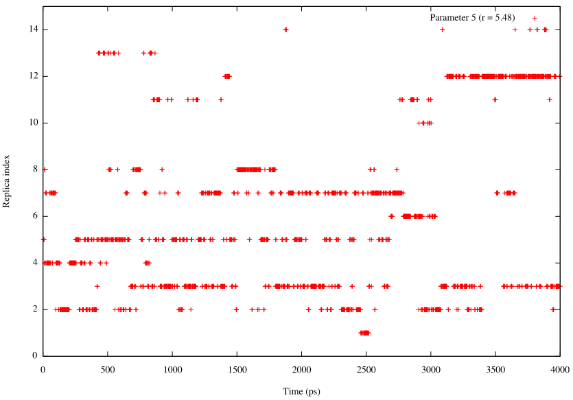
To examine a random walk of the system in the replica space, we analyze the time courses of the replica index. We need to plot one column in the “ParmIDtoRepID:” lines in step4.log on the time axis. Following commands are example to plot the replica index that has Parameter 5 (k = 1.2 kcal/mol/Å2 and r = 5.48Å) during the simulation:
# change directory
$ cd 4_plot_index

# create log file that contains replica index by the grep and cut commands
$ grep "ParmIDtoRepID:" ../../4_production/step4.log | cut -c 17- > id.log

# create log file that contains exchange-attempt step number
$ grep "REMD> Step:" ../../4_production/step4.log | cut -c 12-25 > step.log

# combine step.log and id.log by the paste command
$ paste step.log id.log > index.log

# plot the time courses of replica index that has Parameter 5 (r = 5.48)
$ gnuplot
gnuplot> set xlabel 'Time (ps)'
gnuplot> set ylabel 'Replica index'
gnuplot> plot [][0:15]'index.log' u ($1*2/1000):6 t "Parameter 5 (r = 5.48)"
We also plot the time courses of the target distance of the restraint function in one replica. Because in the log file parameter index is output in the “Parameter :” lines instead of the target distance, we should convert the index to the actual distance value. Here, we use a sed command and script (./script/sed.inp) to convert. Following commands are example to plot the target distance in Replica 8:
# create log file that contains target distance
# sed script is used to convert parameter index to target distance
$ grep "Parameter    :" ../../4_production/step4.log | cut -c 17- > param.log
$ sed -f ./script/sed.inp param.log > dist.log

# combine step.log and dist.log by the paste command
$ paste step.log dist.log > distance.log

# plot the time courses of target distance in Replica 8
$ gnuplot
gnuplot> set xlabel 'Time (ps)'
gnuplot> set ylabel 'Target distance (A)'
gnuplot> plot [][0:15]'distance.log' u ($1*2/1000):9 t "Replica 8" w lines
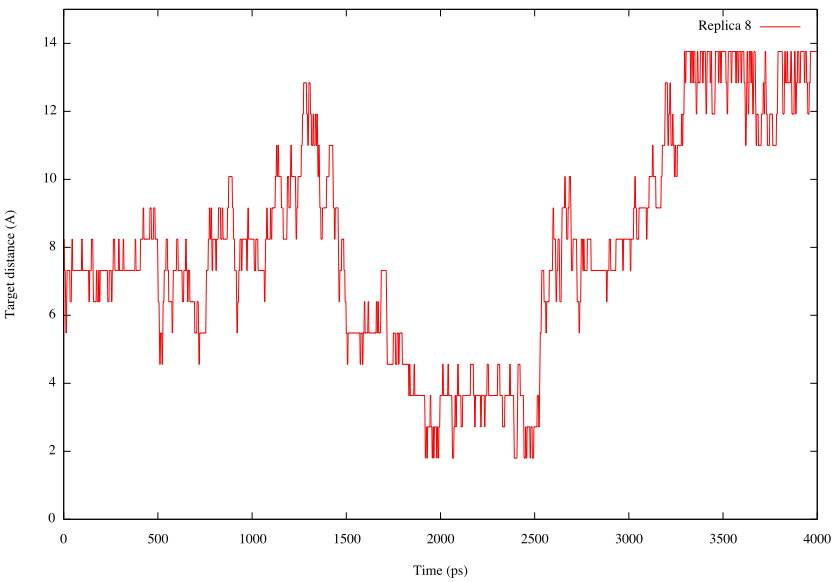
From these plots, we can see that random walk of the system is realized in the REUS simulation.
5. Analyze the end-to-end distance of alanine tripeptide
In this subsection, we calculate the end-to-end distance of the alanine tripeptide by using trj_analysis of the GENESIS analysis tool set. In the 5_calc_dist directory, we have two directories: replica and parameter. The former is used to analyze the original DCD files (../1_convert_dcd/step4_rep{}.dcd), and the latter is used to analyze the sorted DCD files (../2_sort_dcd/step4_par{}.dcd).
# change directory
$ cd 5_calc_dist
$ ls
parameter  replica
First, let us calculate the end-to-end distance of the peptide in the original DCD file. Sample control files are already contained in the directory. Note that we should prepare 14 individual control files to analyze each replica.
# change directory
$ cd replica
$ ls
INP1   INP11  INP13  INP2  INP4  INP6  INP8  run.csh
INP10  INP12  INP14  INP3  INP5  INP7  INP9  script

# check one control file
$ less INP1
[INPUT]
reffile = ../../1_convert_dcd/step4_rep1.pdb  # PDB file

[OUTPUT]
disfile = replica1.dis                        # distance file

[TRAJECTORY]
trjfile1       = ../../1_convert_dcd/step4_rep1.dcd  # trajectory file
md_step1       = 2000000   # number of MD steps
mdout_period1  = 50        # MD output period
ana_period1    = 50        # analysis period
repeat1        = 1
trj_format     = DCD       # (PDB/DCD)
trj_type       = COOR+BOX  # (COOR/COOR+BOX)
trj_natom      = 0         # (0:uses reference PDB atom count)
[OPTION]
check_only     = NO
distance1      = PROA:1:ALA:OY PROA:3:ALA:HNT
INP1 is used to analyze ../../1_convert_dcd/step4_rep1.dcd. Because the DCD file should contain the same number and order of atoms with the input PDB file, we specify ../../1_convert_dcd/step4_rep1.pdb as reffile. In the [TRAJECTORY] section, md_step1 and mdout_period1 correspond to nsteps and crdout_period, respectively, specified in the [DYNAMICS] section of the REUS simulation. If we set mdout_period1 = ana_period1, trajectory data is analyzed every step. Here, we analyze the distance between OY atom in ALA1 and HNT atom in ALA3. After running trj_analysis for INP1 to INP14, we obtain replica1.dis to replica14.dis. We plot the time courses of the distance in Replica 8 below as an example.
# run trj_analysis to analyze the distance
# this is done for 1 to 14 (./run.csh is available for scripting)
$ /home/user/genesis/bin/trj_analysis INP1 > log1
$ /home/user/genesis/bin/trj_analysis INP2 > log2
:
$ /home/user/genesis/bin/trj_analysis INP14 > log14
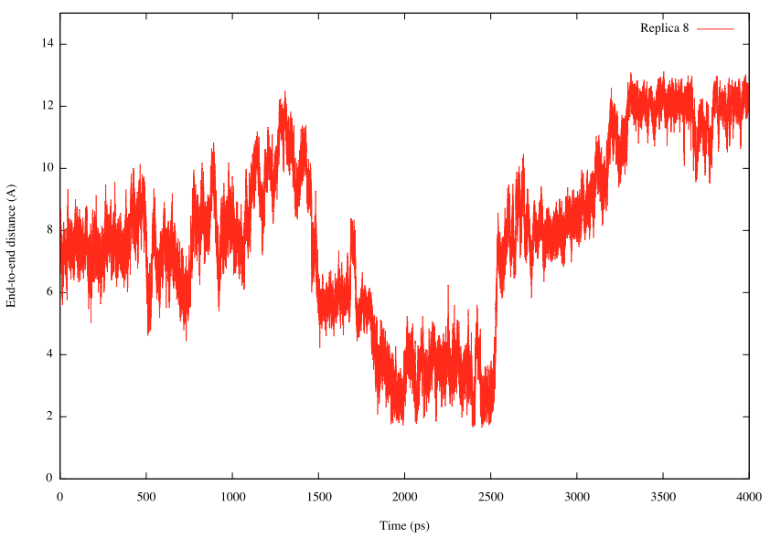
Let us compare the results with the above plot (changes in the target distance in Replica 8). We can see that the distance increases as the target distance increases, and vice versa.
Next, let us calculate the end-to-end distance in the sorted DCD files. Sample control files are already contained in the ./5_calc_dist/parameter directory. Again, we should prepare 14 individual control files to analyze each DCD file. After running trj_analysis, we obtain parameter1.dis to parameter14.dis as the output files. We plot the histogram of the end-to-end distance obtained in each restraint condition by using gnuplot. There are 40,000 distance data in each file, and we set the bin width to be 0.05Å.
# change directory
$ cd ../parameter
$ ls
INP1   INP11  INP13  INP2  INP4  INP6  INP8  run.csh
INP10  INP12  INP14  INP3  INP5  INP7  INP9  script

# run trj_analysis to analyze the distance
$ /home/user/genesis/bin/trj_analysis INP1 > log1
$ /home/user/genesis/bin/trj_analysis INP2 > log2
:
$ /home/user/genesis/bin/trj_analysis INP14 > log14

# plot the histogram of the end-to-end distance
$ gnuplot
gnuplot> set key outside
gnuplot> set xlabel 'Distance (A)'
gnuplot> set ylabel 'Probability'
gnuplot> binwidth=0.05
gnuplot> bin(x,width)=width*floor(x/width)
gnuplot> ndata=40000
gnuplot> plot for [k=1:14] "parameter".k.".dis" u (bin($2,binwidth)):(1.0/ndata) t "Parameter".k smooth freq
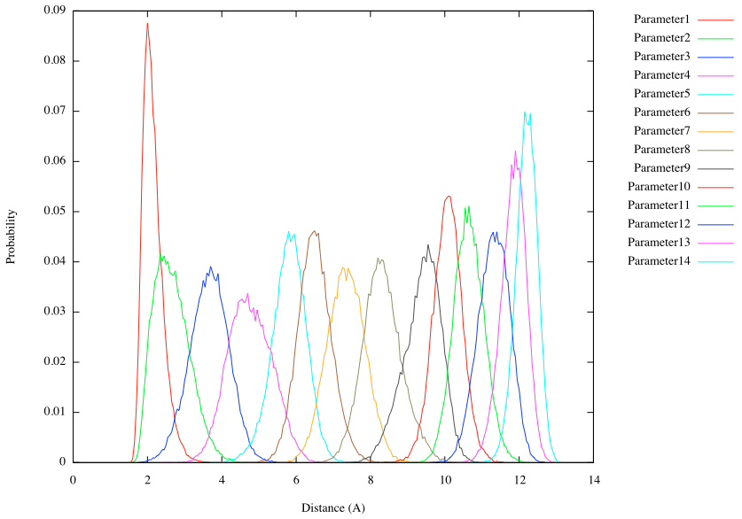
The results show that there is enough overlap between neighboring umbrella windows along the reaction coordinates. These overlaps are important to obtain reliable free energy profile in the subsequent WHAM technique.
6. Free energy calculation using WHAM
We calculate the free energy profile of the alanine tripeptide as a function of the end-to-end distance by using WHAM. Here, we use wham_analysis of the GENESIS analysis tool set. Let us move to the 6_calc_wham directory, and see the sample control file:
# change directory
$ cd 6_calc_wham
$ less INP
[INPUT]
cvfile         = ../5_calc_dist/parameter/parameter{}.dis

[OUTPUT]
pmffile        = output.pmf     # potential of mean force file

[WHAM]
dimension      = 1
temperature    = 300.0
tolerance      = 10E-08
rest_function1 = 1
grids1         = 0.0 15.0 301   # min, max, and num_grids (number of bins + 1)

[RESTRAINTS]
constant1      = 1.2 1.2 1.2 1.2 1.2 1.2 1.2 1.2 1.2 1.2 1.2 1.2 1.2 1.2
reference1     = 1.80  2.72  3.64  4.56  5.48  6.40  7.32  \
                 8.24  9.16 10.08 11.00 11.92 12.84 13.76
is_periodic1   = NO
In the [INPUT] section, we specify the output file generated from the distance analysis for the sorted DCD files (see the previous subsection). In the [WHAM] section, we set the number of the dimension of the reaction coordinates, temperature used in the REUS simulation, tolerance of the WHAM iteration, number of grids in the PMF profile, and so on. For the [RESTRAINTS] section, we give the same information used in the REUS control file.
# perform wham
$ /home/user/genesis/bin/wham_analysis INP > log

# plot the free energy profile
$ gnuplot
gnuplot> set xlabel 'Distance (A)'
gnuplot> set ylabel 'Potential of mean force (kcal/mol)'
gnuplot> plot [0:14][0:10]'output.pmf' w lines
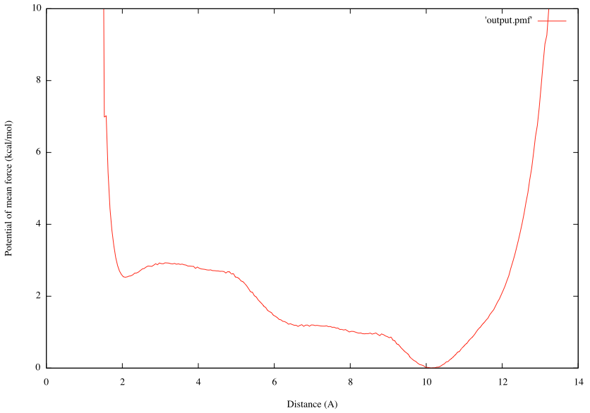
We can see that there is the global energy minimum at r = 10.13Å and a local energy minimum at r = 2.08Å. The latter corresponds to the α-helix conformation, where the hydrogen bond between OY and HNT is formed. These results suggest that in water the alanine tripeptide tends to form an extended conformation rather than α-helix with the free energy difference of ~2.5 kcal/mol.
If you utilize other WHAM tools, pay attention to the equation of the umbrella potential. In GENESIS, both REUS simulation and WHAM analysis use k*(r – r0)2 for the umbrella, while other programs might be using k/2*(r – r0)2.
Written by Takaharu Mori@RIKEN Theoretical molecular science laboratory
July, 13, 2016