4.4 Principal component analysis (PCA)
Files for this tutorial (tutorial-4.4.tar.gz)
In this tutorial, we perform principal component analysis (PCA). PCA is useful to understand the dynamical behaviour of biomolecules by projecting the trajectory on small dimensions in terms of principal components (PCs). To perform PCA, we first use the eigmat_analysis tool, followed by the prjcrd_analysis tool, both of which are available in the GENESIS analysis tool sets. The former computes the eigenvalue and eigenvectors of the variance-covarience matrix, and the latter carries out a projection of the snapshot structures onto PC vectors.
In this tutorial, we use the output files obtained in tutorial 1.1 and tutorial 4.3. (Please work on these tutorials first if you have not done it yet.) Untar tutorial-4.4.tar.gz in the same directory as tutorial-1.1 and tutorial-4.3:
$ ls
tutorial-1.1  tutorial-4.3
$ tar -zxf tutorial-4.4.tar.gz
$ ls
tutorial-1.1  tutorial-4.3  tutorial-4.4
$ cd tutorial-4.4
$ ls
run.sh  run1.inp  run2.inp
In tutorial-1.1, we carried out an MD simulation of a small protein, BPTI, in solution. The MD simulation was performed for 500,000 steps with crdout_period = 500, resulting in a trajectory file containing 1,000 snapshots. In tutorial-4.3, we analyzed RMSF of all residues in BPTI. Here, we calculate the PCs of BPTI and project all snapshots of the trajectory on to a plane of two PCs.
The control file, run1.inp, is for eigmat_analysis:
[INPUT]
pcafile = ../tutorial-4.3/run2.pca # PCA file

[OUTPUT]
valfile = run1.val   # VAL file
vecfile = run1.vec   # VEC file
cntfile = run1.cnt   # CNT file
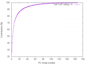
We obtain valfile, vecfile, and cntfile, which contain eigenvalues, eigenvectors, and contribution of each mode to the overall dynamics, respectively. The following figure shows the plot of the accumulated contribution of each PC mode (4th column in cntfile).
The control file, run2.inp, for prjcrd_analysis is as follows:
[INPUT]
reffile     = ../tutorial-1.1/1_setup/ionize.pdb    # PDB file
pdb_avefile = ../tutorial-4.3/run1_ave.pdb  # PDB file (Average coordinates)
pdb_aftfile = ../tutorial-4.3/run1_aft.pdb  # PDB file (Fitted Average coordinates)
valfile     = run1.val # VAL file
vecfile     = run1.vec # VEC file

[OUTPUT]
prjfile     = run2.prj # PRJ file
In [INPUT] section, reffile is the reference structure used in tutorial-1.1, and pdb_avefile and pdbaftfile are the average coordinates of the analysis and fitting atoms, respectively, obtained in tutorial-4.3. valfile and vecfile are the output of eigmat_analysis.
[TRAJECTORY], [SELECTION], and [FITTING] sections, which follow the above, are the same as before. See tutorial-4.1 for details.
[OPTION]
check_only     = NO       # (YES/NO)
vcv_matrix     = Global   # (GLOBAL/LOCAL)
num_pca        = 2        # # of principal components
analysis_atom  = 1        # analysis target atom group
In [OPTION] section, we specify the number of PCs to project the trajectory. The PCs are selected in a decreasing order of their contributions.
The analysis is executed by run.sh script:
$ cat run.sh
#!/bin/bash

# set the number of OpenMP threads
export OMP_NUM_THREADS=1

# perform analysis with eigmat_analysis and prjcrd_analysis
$ eigmat_analysis run1.inp | tee run1.out
$ prjcrd_analysis run2.inp | tee run2.out
Now, let’s run the script:
$ chmod +x run.sh
$ ./run.sh
$ ls
run.sh    run1.cnt  run1.inp  run1.out  run1.val
run1.vec  run2.inp  run2.out  run2.prj
We obtain run2.prj which contains the projection of each structure onto the calculated principal component axes. The i-th principal component μi of each snapshot is defined by the dot product:
\( \displaystyle \mu_i = \mathbf{v}_i \cdot (\mathbf{q}- \langle \mathbf{q} \rangle) \)
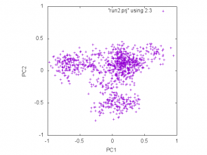
where \(\displaystyle \mathbf{v}_i \) is the i-th eigenvector, q is the coordinates of each snapshot in the trajectory, and \( \langle \mathbf{q} \rangle \) is the
averaged coordinates. The following figure is the plot of 2nd and 3rd columns of run2.prj:
$ gnuplot
gnuplot> set xlabel "PC1"
gnuplot> set ylabel "PC2"
gnuplot> set xrange [-1:1]
gnuplot> set yrange [-1:1]
gnuplot> set size square
gnuplot> plot "run2.prj" using 2:3
Written by Kiyoshi Yagi@RIKEN Theoretical molecular science laboratory
July, 17, 2016