4.3 Root-mean-square fluctuation (RMSF)
Files for this tutorial (tutorial-4.3.tar.gz)
In this tutorial, we analyze the root-mean-square fluctuation (RMSF). To compute the RMSF, we first use the avecrd_analysis tool, followed by the flccrd_analysis tool, both of which are available in the GENESIS analysis tool sets. The former computes the averaged coordinates of the selected atoms, and the latter computes the RMSF.
In this tutorial, we use the output files obtained in tutorial 1.1. (Please work on tutorial 1.1 first if you have not done it yet.) Untar tutorial-4.3.tar.gz in the same directory as tutorial-1.1:
$ ls
tutorial-1.1
$ tar -zxf ~/Download/tutorial-4.3.tar.gz
$ ls
tutorial-1.1 tutorial-4.3
$ cd tutorial-4.3
$ ls
run.sh  run1.inp  run2.inp
In tutorial-1.1, we carried out an MD simulation of a small protein, BPTI, in solution. The MD simulation was performed for 500,000 steps with crdout_period = 500 resulting in a trajectory file containing 1,000 snapshots. Here, we analyze RMSF of Cα atoms in BPTI for all snapshots.
The control file, run1.inp, is for avecrd_analysis. Let’s look into this file.
[INPUT]
reffile        = ../tutorial-1.1/1_setup/ionize.pdb    # PDB file

[OUTPUT]
pdbfile        = run1.pdb        # PDB file
rmsfile        = run1.rms        # RMSD file
pdb_avefile    = run1_ave.pdb    # PDB file (Averaged coordinates of analysis atoms)
pdb_aftfile    = run1_aft.pdb    # PDB file (Averaged coordinates of fitting atoms)

[TRAJECTORY]
trjfile1       = ../tutorial-1.1/5_production/run.dcd  # trajectory file
md_step1       = 500000          # number of MD steps
mdout_period1  =    500          # MD output period
ana_period1    =    500          # analysis period
repeat1        = 1
trj_format     = DCD             # (PDB/DCD)
trj_type       = COOR            # (COOR/COOR+BOX)
trj_natom      = 0               # (0:uses reference PDB atom count)

[SELECTION]
group1         = an:CA           # selection group 1

[FITTING]
fitting_method = TR+ROT          # method
fitting_atom   = 1               # atom group
mass_weight    = YES             # mass-weight is applied

[OPTION]
check_only     = NO              # (YES/NO)
num_iterations = 10              # number of iterations
analysis_atom  = 1               # analysis target atom group
In [OUTPUT] section, pdb_avefile and pdb_aftfile are the name of output PDB files that contain averaged coordinates of analysis atoms and averaged coordinates of fitting atoms, respectively. The averaged coordinates of the selected atoms are computed iteratively based on num_iterations in [OPTION] section.
Other options are the same as the input for computing the RMSD in tutorial-4.1.
The control file, run2.inp, is for flccrd_analysis. It is almost the same as run1.inp except for:
[INPUT]
reffile        = ../tutorial-1.1/1_setup/ionize.pdb    # PDB file
pdb_avefile    = run1_ave.pdb    # PDB file (Average coordinates)
pdb_aftfile    = run1_aft.pdb    # PDB file (Fitted Average coordinates)

[OUTPUT]
pcafile        = run2.pca        # PCA file
rmsfile        = run2.rms        # RMSF and B-factor file
vcvfile        = run2.vcv        # Variance-Covarience Matrix file
crsfile        = run2.crs        # CRS file
In [INPUT] section, we read pdb_avefile and pdb_aftfile obtained from avecrd_analysis. In the [OUTPUT] section, we specify the files to which the output data are written. RMSF is written in rmsfile. pcafile is needed for the principal component analysis in tutorial-4.4.
The analysis is executed by run.sh script:
$ cat run.sh
#!/bin/bash

# set the number of OpenMP threads
export OMP_NUM_THREADS=1

# perform analysis with avecrd_analysis and flccrd_analysis
avecrd_analysis run1.inp | tee run1.out
flccrd_analysis run2.inp | tee run2.out
Now, let’s execute this file:
$ chmod +x run.sh
$ ./run.sh
$ ls
run.sh    run1.out  run1.rms      run1_ave.pdb  run2.inp  run2.pca  run2.vcv
run1.inp  run1.pdb  run1_aft.pdb  run2.crs      run2.out  run2.rms
In run2.rms, the 4th column corresponds to RMSF in the unit of Angstrom, and the 5th column is the B-factor calculated from RMSF. This can be plotted with gnuplot:
$ gnuplot
gnuplot> set xlabel "Residue number"
gnuplot> set ylabel "RMSF [angstrom]"
gnuplot> plot "run2.rms" using 1:4 w lp
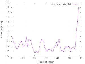
We can see that the RMSF for the loop regions are larger than the residues forming the helix and sheet conformations, indicating that the secondary structures make the protein rigid.
Written by Kiyoshi Yagi@RIKEN Theoretical molecular science laboratory
July, 18, 2016