4.1 Root-mean-square deviation (RMSD)
Files for this tutorial (tutorial-4.1.tar.gz)
In this tutorial, we use rmsd_analysis in GENESIS analysis tool sets to calculate the root-mean-square deviation (RMSD) of the target molecule with respect to a reference structure. The RMSD is given by
\( \displaystyle RMSD = \sqrt{\frac{1}{n} \sum_{i=1}^{n} (x_i – x_{i0})^2 + (y_i – y_{i0})^2 + (z_i – z_{i0})^2 } \)
where \(n\) is the number of atoms and \((x_{i0}, y_{i0}, z_{i0})\) is the coordinates of the reference structure.
In this tutorial, we use the output files obtained in tutorial 1.1. (Please work on tutorial 1.1 first if you have not done it yet.) Untar tutorial-4.1.tar.gz in the same directory as tutorial-1.1:
$ ls
tutorial-1.1
$ tar -zxf ~/Download/tutorial-4.1.tar.gz
$ ls
tutorial-1.1 tutorial-4.1
$ cd tutorial-4.1
$ ls
run.inp run.sh
In tutorial-1.1, we carried out an MD simulation of a small protein, BPTI, in solution. The MD simulation was performed for 500,000 steps with crdout_period = 500, resulting in a trajectory file containing 1,000 snapshots. Here, we analyze RMSD of Cα atoms in BPTI for all snapshots with respect to the initial structure.
In this tutorial, run.inp is the control file. Let’s look into this file.
[INPUT]
reffile = ../tutorial-1.1/1_setup/ionize.pdb  # PDB file

[OUTPUT]
rmsfile        = run.rms # RMSD file
In [INPUT] section, reffile option is the reference structure for calculating the RMSD. Here, it is the crystal structure, which we downloaded from the Protein Data Bank (PDBID: 4pti). In [OUTPUT] section, we specify the name of the output by rmsfile = run.rms, where the RMSD of each snapshot will be written.
[TRAJECTORY]
trjfile1       = ../tutorial-1.1/5_production/run.dcd # trajectory file
md_step1       = 500000  # number of MD steps
mdout_period1  = 500     # MD output period
ana_period1    = 500     # analysis period
repeat1        = 1
trj_format     = DCD     # (PDB/DCD)
trj_type       = COOR    # (COOR/COOR+BOX)
trj_natom      = 0       # (0:uses reference PDB atom count)
Input trajectory file is specified with trjfile1 in the [TRAJECTORY] section. md_step1 and mdout_period1 are, respectively, nsteps and crdout_period specified in the MD simulation. To know more about how to deal with this section, see here.
[SELECTION]
group1         = an:CA   # selection group 1

[FITTING]
fitting_method = TR+ROT  # method
fitting_atom   = 1       # atom group

[OPTION]
check_only     = NO      # (YES/NO)
analysis_atom  = 1       # atom group
In the [SELECTION] section, the group of atoms that is used for structure fitting and RMSD analysis is defined. Here, we select Cα atoms of the protein. In the [FITTING] section, the method for structure fitting is specified. In this example, fitting by translation TR and rotation ROT is used. In the [OPTION] section, if check_only = YES is specified, the program just checks input files without doing any analysis.
fitting_atom in the [FITTING] section and analysis_atom in the [OPTION] section are an index for a group of atoms for structure fitting and RMSD analysis, respectively. The index is specified in the [SELECTION] section. The user can specify different group indices for fitting_atom and analysis_atom; see below for details.
rmsd_analysis is executed by run.sh script:
$ cat run.sh
#!/bin/bash

rm -i run.rms

# set the number of OpenMP threads
export OMP_NUM_THREADS=1

# perform rmsd analysis
rmsd_analysis run.inp | tee run.out
Note that the output file is not overwritten as in other GENESIS programs. So, a file with the same name must NOT exist in the same directory.
Now, let’s run rmsd_analysis:
$ chmod +x run.sh
$ ./run.sh
$ ls
run.inp   run.out   run.rms   run.sh
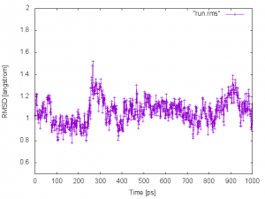
We obtain run.rms. In the file, the first column is the index of a snapshot, and the second column is the RMSD values in the Angstrom unit. This can be plotted with gnuplot:
$ gnuplot
gnuplot> set xlabel "Time [ps]"
gnuplot> set ylabel "RMSD [angstrom]"
gnuplot> set yrange [0.5:2.0]
gnuplot> plot "run.rms" w lp
The user can specify fitting_atom and analysis_atom individually. For example, in protein-ligand system, RMSD of ligand with respect to protein can be analyzed by specifying fitting_atom to be the protein and analysis_atom to be the ligand. An example of the control file is as follows:
[SELECTION]
group1         = ai:1-1600            # protein atoms
group2         = ai:1601-1700         # ligand atoms

[FITTING]
fitting_method = TR+ROT               # method
fitting_atom   = 1                    # atom group

[OPTION]
analysis_atom  = 2                    # atom group
Written by Takaharu Mori@RIKEN Theoretical molecular science laboratory
Updated by Kiyoshi Yagi@RIKEN Theoretical molecular science laboratory
July, 15, 2016