6.1 POPC lipid bilayers with the CHARMM force field
Contents
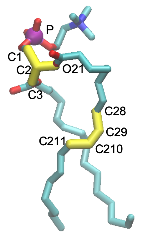
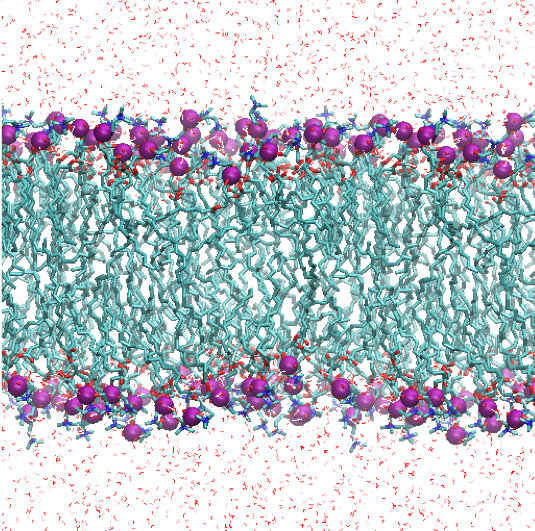
One of the widely used models for biological membranes is a bilayer of POPC (1-palmitoyl-2-oleoyl-sn-glycero-3-phosphocholine) lipids. The chemical formula of POPC is shown below. It consists of hydrophobic tail groups and hydrophilic head groups. In POPC, one of the fatty acid tails has a double bond with a cis conformation, and there is a stereocenter in the middle (both indicated in red in the figure). Because of its amphiphilic character, POPC lipids self-assemble to form a bilayer structure.
The aim of this tutorial is to learn:
- How to prepare an all-atom model for a POPC bilayer.
- How to equilibrate the POPC bilayer system.
- How to generate an MD trajectory and perform analyses on it.
In this tutorial, we carry out all-atom MD simulations of a lipid bilayer with GENESIS and CHARMM-GUI using the CHARMM36 force field [1].
1. Preparation
Let’s download the tutorial file (tutorial-6.1.zip). This tutorial consists of four steps: 1) system setup using CHARMM-GUI, 2) energy minimization and equilibration, 3) production run, and 4) trajectory analysis. Since we use the CHARMM force field, we make a symbolic link to the CHARMM toppar directory (see Tutorial 2.2).
# Download the tutorial file
$ cd ~/GENESIS_Tutorials-2022/Works
$ mv ~/Downloads/tutorial22-6.1.zip ./
$ unzip tutorial22-6.1.zip
$ cd tutorial-6.1

# Clean up the working directory
$ mv tutorial22-6.1.zip ./TRASH

# Let's take a note
$ echo "tutorial-6.1: MD simulation of a POPC lipid bilayer" >> README

# Make a symbolic link to the CHARMM toppar directory
$ cd tutorial22-6.1
$ ln -s ../../Data/Parameters/toppar_c36_jul21 ./toppar
$ ls
1_charmm-gui  2_min_equil  3_production  4_analysis  toppar
2. Setup initial structure with CHARMM-GUI
One of the difficulties is the setup of a bilayer structure. Because each lipid molecule has a random structure, it takes much time to equilibrate the whole system, if one starts the simulation from an ordered structure. CHARMM-GUI is one of the useful tools to generate initial structures of a lipid bilayer for MD simulations [2]. It provides an automatic membrane builder not only for lipid bilayers but also for protein-membrane systems.
In case the server is down, you can skip this section and use the files included in the folder 1_charmm-gui, which we obtained from CHARMM-GUI.
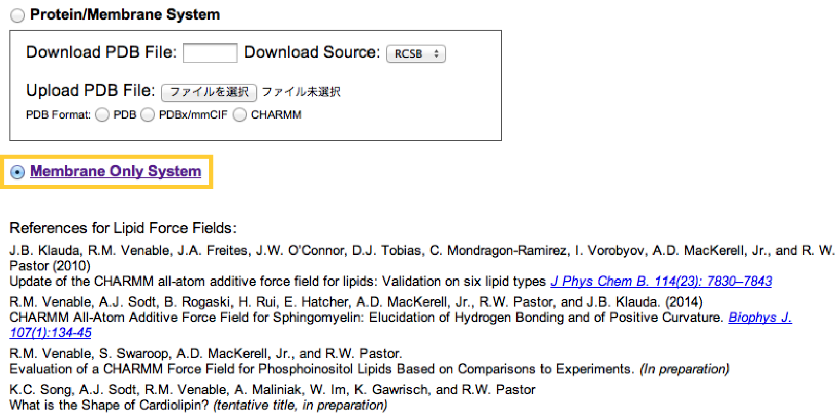
Click [here] to access CHARMM-GUI top page. You will need to log in or register in case you have an account. The Bilayer builder can be accessed from the top page, Input Generator, Membrane Builder, and then Bilayer Builder. At the first step of the bilayer builder, we choose “Membrane Only System”:
 In the next step, we decide the number of lipids and water molecules to be added to the system. Here, we put 40 POPC and 40 POPC lipids in the upper and lower leaflets, respectively (Note that these numbers might be a lower limit for stable MD simulations with
 spdyn). Because each lipid molecule has a certain area per lipid (Aexp = 68.3Å2 for POPC), the initial box size (X, Y) = (52.27Å, 52.27Å) can be estimated from \(X=Y=\sqrt{n \times A}\), where \(n\) is the number of lipids in one leaflet and \(A\) is the area per lipid in Å2 (assuming both leaflets have the same composition and the same number of lipids).
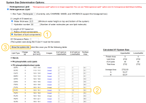
Note that one may alternatively choose “Ratios of lipid components”, set “Length of X and Y”, and set “Upperleaflet Ratio” and “Lowerleaflet Ratio” for each lipid. This scheme is useful for building mixed lipid systems.
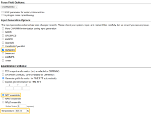
In the next step, we add 0.15 M KCl to the system, mimicking the cellular environment, with the Monte Carlo method for ion placing. Then, we click “Next Step” and continue to Step5. We check “GENESIS” in “Input Generation Options” and select the NPT ensemble at T = 303.15 K in “Equilibration Options”. At this temperature, the POPC bilayer is in the liquid phase rather than the gel phase (Tm = 271 K). After clicking “Next Step”, we can download a set of input files for minimization, equilibration, and production runs at the final step of the membrane builder. The download begins when you click a “download.tgz” button in the upper right corner.
After the download, let’s check the structure of the downloaded PDB file using VMD:
# move the downloaded tar file and untar
$ mv ~/Download/charmm-gui.tgz ./
$ tar -xzf charmm-gui.tgz
$ ls
1_charmm-gui/ 3_production/ charmm-gui-XXXXXXXXXXXX/
2_min_equil/ 4_analysis/ charmm-gui.tgz

# Check the final pdb file
$ cd charmm-gui-XXXXXXXXXXXX
$ vmd step5_assembly.pdb
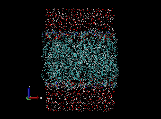
“XXXXXXXXXX” is a 10-digit ID number given by the CHARMM-GUI sever. Visually check that the system is constructed as you intended (the type of lipids, number of lipids, etc.). Note that the membrane normal is taken to be the z-axis, which is the convention in the field. You may also check step5_assembly.str, where the box size, the number of water molecules, and other information about the system are found. If no serious problem is found, we use the PDB file and an associated PSF file (step5_assembly.psf) as the initial coordinates and topology for the simulation, respectively. Rename the downloaded folder to 1_charmm-gui,
# Save the original folder, and rename the new one
$ cd ..
$ mv 1_charmm-gui 1_charmm-gui.org
$ mv charmm-gui-XXXXXXXXXXXX 1_charmm-gui
$ ls
1_charmm-gui/ 1_charmm-gui.org/ 3_production/
2_min_equil/ 4_analysis/ charmm-gui.tgz
Auto-generated control files for GENESIS are also contained in 1_charmm-gui/genesis:
$ ls ./1_charmm-gui/genesis
restraints/        step6.0_minimization.inp     step6.4_equilibration.inp    sysinfo.dat
step5_input.crd    step6.1_equilibration.inp    step6.5_equilibration.inp
step5_input.pdb    step6.2_equilibration.inp    step6.6_equilibration.inp
step5_input.psf    step6.3_equilibration.inp    step7_production.inp
However, in this tutorial, we will use a slightly modified version of these files to take advantage of GENESIS 2.0 latest features.
3. Minimization and Equilibration
Let’s move to 2_min_equil and find control files for minimization (step6.0) and equilibration (step6.1 – 6.6),
$ cd ./2_min_equil
$ ls
equil.vmd        restraints/                step6.1_equilibration.inp  step6.4_equilibration.inp
equil_area.gpi   run.sh                     step6.2_equilibration.inp  step6.5_equilibration.inp
equil_temp.gpi   step6.0_minimization.inp   step6.3_equilibration.inp  step6.6_equilibration.inp
Note that psffile, pdbfile, and reffile are set to the files in 1_charmm-gui,
psffile = ../1_charmm-gui/step5_assembly.psf  # protein structure file
pdbfile = ../1_charmm-gui/step5_assembly.pdb  # PDB file
reffile = ../1_charmm-gui/step5_assembly.pdb  # reference PDB file for restraint
The control files for minimization and equilibration are almost the same as before [see Sec. 3.2]. The difference is in the way restraints are applied.
3.1. The restraints for POPC
The dihedral angles, C3-C1-C2-O21 and C28-C29-C210-C211 (shown in yellow in the figure below) are restrained to 120 and 0 degrees, respectively, to keep the stereoisomer and the cis-isomer. Furthermore, the position of a phosphate atom, (shown in purple), is also restrained in the Z direction to keep the thickness of the bilayer.
The dihedral angles are restrained using localresfile in the [INPUT] section. For example, step6.0_minimization.inp is as follows,
[INPUT]
topfile = ../toppar/top_all36_lipid.rtf             # topology file
parfile = ../toppar/par_all36_lipid.prm             # parameter file
strfile = ../toppar/toppar_water_ions.str           # stream file
psffile = ../1_charmm-gui/step5_assembly.psf        # protein structure file
pdbfile = ../1_charmm-gui/step5_assembly.pdb        # PDB file
reffile = ../1_charmm-gui/step5_assembly.pdb        # reference PDB file for restraint
localresfile = restraints/step6.0_minimization.dihe # local restraint file
localresfile lists the dihedral angles in the following format,
DIHEDRAL 60 63 65 67 250 0.0
DIHEDRAL 36 25 28 30 250 120.0
DIHEDRAL 194 197 199 201 250 0.0
...
The first line means that a dihedral angle of atom index, 60-63-65-67, (i.e. C28-C29-C210-C211 of the first POPC) is restrained to 0.0 degree with a force constant of 250 kcal/mol. Similarly, the second line restrains C3-C1-C2-O21 of the first POPC to 120.0 degrees with the same force constant. The restraints for other POPCs follow in the file.
The positional restraint of phosphate atoms is specified in the control file by [RESTRAINTS] and [SELECTION] sections,
[SELECTION]
group1           = sid:MEMB and ((rnam:POPC and (an:P)))  # restriant group 1

[RESTRAINTS]
nfunctions       = 1       # number of functions
function1        = POSI    # restraint function type
direction1       = Z       # direction [ALL,X,Y,Z]
constant1        = 2.5     # force constant
select_index1    = 1       # restrained groups
Note that the direction is set along the Z axis. Thus, POPC can move freely in the membrane plane, and be restrained in the direction of the membrane normal.
3.2. Run GENESIS
The setting of each step is summarized in the following table:
| Step | Ensemble | Integrator | Step | dt / fs | Time / ps | k [dihed] | k [Pz] |
| 0 | Min | – | 2,000 | – | – | 250 | 2.5 |
| 1 | NVT | VVER | 25,000 | 1 | 25 | 250 | 2.5 |
| 2 | NVT | VVER | 25,000 | 1 | 25 | 100 | 2.5 |
| 3 | NPT | VVER | 25,000 | 1 | 25 | 50 | 1.0 |
| 4 | NPT | VVER | 50,000 | 2 | 100 | 50 | 0.5 |
| 5 | NPT | VVER | 50,000 | 2 | 100 | 25 | 0.1 |
| 6 | NPT | VRES | 40,000 | 2.5 | 100 | 0 | 0 |
Note that the force constants (k [dihed] and k[Pz]) are gradually reduced. Also, the timestep, which is initially set to 1 fs, is increased to 2 fs and 2.5 fs in the last step. Step 6 is carried out with the RESPA integrator.
The simulation with NPT is carried out with the semi-iso option, which keeps the ratio of the box size in the x and y directions,
[ENSEMBLE]
ensemble         = NPT      # [NVE,NVT,NPT]
tpcontrol        = BUSSI    # thermostat and barostat
temperature      = 303.15   # initial and target temperature (K)
pressure         = 1.0      # atm
isotropy         = SEMI-ISO # keep the ratio of X and Y
Let’s execute GENESIS. run.sh is a script to run SPDYN for all steps:
$ cat run.sh
#!/bin/bash

spdyn=../../../Programs/genesis-2.0/bin/spdyn

# 2000 step energy minimization
# with dihedral angle restraint (k = 250 kcal/mol)
#      z-positional restraint on P atoms (k = 2.5 kcal/mol/Angs^2)
export OMP_NUM_THREADS=1
mpirun -np 16 $spdyn step6.0_minimization.inp >& log6.0

# 25ps MD in the NVT ensemble
# with dihedral angle restraint (k = 250 kcal/mol)
#      z-positional restraint on P atoms (k = 2.5 kcal/mol/Angs^2)
mpirun -np 16 $spdyn step6.1_equilibration.inp >& log6.1

# 25ps MD in the NVT ensemble
# with dihedral angle restraint (k = 100 kcal/mol)
#      z-positional restraint on P atoms (k = 2.5 kcal/mol/Angs^2)
mpirun -np 16 $spdyn step6.2_equilibration.inp >& log6.2

# 25ps MD in the NPT ensemble
# with dihedral angle restraint (k = 50 kcal/mol)
#      z-positional restraint on P atoms (k = 1.0 kcal/mol/Angs^2)
mpirun -np 16 $spdyn step6.3_equilibration.inp >& log6.3

# 100ps MD in the NPT ensemble
# with dihedral angle restraint (k = 50 kcal/mol)
#      z-positional restraint on P atoms (k = 0.5 kcal/mol/Angs^2)
mpirun -np 16 $spdyn step6.4_equilibration.inp >& log6.4

# 100ps MD in the NPT ensemble
# with dihedral angle restraint (k = 25 kcal/mol)
#      z-positional restraint on P atoms (k = 0.1 kcal/mol/Angs^2)
mpirun -np 16 $spdyn step6.5_equilibration.inp >& log6.5

# 100ps MD in the NPT ensemble without any restraints using VRES
mpirun -np 16 $spdyn step6.6_equilibration.inp >& log6.6
Execute this script. This may take about an hour or so.
# Run all steps
$ ./run.sh
When the calculation is done, it is a good practice to check the status before moving on to the production step.
3.3. Check the status: Visualization
$ vmd -e equil.vmd
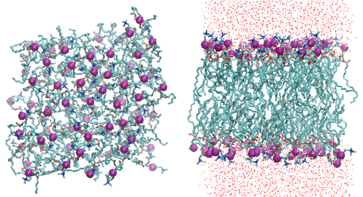
The molecules can be wrapped into a simluation box by typing,
pbc wrap -center com -compound residue -all
in the console of VMD. The console of VMD opens by choosing “Extensions -> Tk Console” in the VMD Main window.
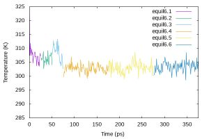
3.4. Check the status: Temperature and Area per lipid (AL)
Extract the “INFO” lines from output files to individual files,
$ for i in 1 2 3 4 5 6; do
grep INFO log6.${i} > energy6.${i}.log
done
Then, plot the temperature data using gnuplot,
$ cat equil_temp.gpi
set terminal jpeg size 600,400
set output 'equil_temp.jpg'

set xlabel 'Time (ps)'
set ylabel 'Temperature (K)'

set xrange [0:375]
set yrange [285:325]

plot 'energy6.1.log' using 3:16 w l t 'equil6.1', \
     'energy6.2.log' using ($3+25):16 w l t 'equil6.2', \
     'energy6.3.log' using ($3+50):16 w l t 'equil6.3', \
     'energy6.4.log' using ($3+75):16 w l t 'equil6.4', \
     'energy6.5.log' using ($3+175):16 w l t 'equil6.5', \
     'energy6.6.log' using ($3+275):16 w l t 'equil6.6'

$ gnuplot equil_temp.gpi
$ eog equil_temp.jpg
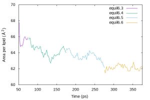
AL is obtained by Lx * Ly / nL, where Lx and Ly are the simulation box size in the x and y dimension, respectively, and nL is the number of lipids in one of the leaflets.
$ cat equil_area.gpi
set terminal jpeg size 600,400
set output 'equil_area.jpg'

set xlabel 'Time (ps)'
set ylabel 'Area per lipid ({\305}^2)'

set xrange [50:375]
set yrange [60:70]

plot 'energy6.3.log' using ($3+50):($18*$19/40) w l t 'equil6.3', \
'energy6.4.log' using ($3+75):($18*$19/40) w l t 'equil6.4',  \
'energy6.5.log' using ($3+175):($18*$19/40) w l t 'equil6.5', \
'energy6.6.log' using ($3+275):($18*$19/40) w l t 'equil6.6'

$ gnuplot equil_area.gpi
$ eog equil_area.jpg
If no serious problem is found, we now continue with the production step.
4. Production
Let’s move to 3_production. In this section, we carry out a NPT simulation for 1 ns. run.sh is a script to run SPDYN:
$cd ../3_production
$ cat run.sh
#!/bin/bash

spdyn=../../../Programs/genesis-2.0/bin/spdyn

# 1000ps MD in the NPT ensemble using VRES
export OMP_NUM_THREADS=1
mpirun -np 16 $spdyn step7_production.inp >& log7
Although the script uses 1 OpenMP thread x 16 MPI processes, it may not be optimal for your computing system. It is highly recommended to benchmark the cost before starting the production run. See Sec. 3.3 for more details.
Execute this script. This may take several hours.
# Run all steps
$ ./run.sh
The trajectory can be visualized by,
$ vmd -e prod.vmd
5. Analysis
Let’s analyze the resulting trajectory. Move to the 4_analysis folder,
$ cd ../4_analysis
$ ls
prod_area.gpi  thickness.gpi  thickness.inp
5.1. Area per lipid (AL)
AL is obtained as before by first extracting the “INFO” lines from the output, and calculating and plotting Lx * Ly / nL with gnuplot,
$ grep INFO ../3_production/log7 > energy7.log
$ cat prod_area.gpi
set terminal jpeg size 800,400
set output 'prod_area.jpg'

set xlabel 'Time (ps)'
set ylabel 'Area per lipid ({\305}^2)'

set xrange [0:1000]
set yrange [60:70]

plot 'energy7.log' using 3:($17*$18/40) w l t 'energy7'

$ gnuplot prod_area.gpi
$ eog prod_area.jpg
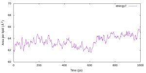
Although the calculated AL is slightly smaller than the experimental value (Aexp = 68.3Å2 for POPC), GENESIS reproduces the averaged area per lipid of 64.7Å2 reported in the CHARMM36 paper [1].
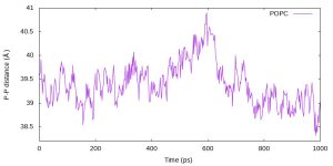
5.2. Bilayer thickness
lipidthick_analysis calculates the average Z-position of specified atoms in the upper and lower leaflets, and gives the membrane thickness as a different between the two. The input file, thickness.inp, looks as follows,
[INPUT]
psffile = ../1_charmm-gui/step5_assembly.psf
reffile = ../1_charmm-gui/step5_assembly.pdb

[OUTPUT]
outfile = thickness.log

[TRAJECTORY]
trjfile1      = ../3_production/step7_production.dcd
md_step1      = 400000
mdout_period1 = 800
ana_period1   = 800
trj_format    = DCD
trj_type      = COOR+BOX

[SELECTION]
group1        = resname:POPC and an:P

[OPTION]
check_only    = NO
membrane_atom = 1     # atom group representing lipid bilayer
- output file is set to thickness.log
- membrane_atom = 1 of [OPTION] and group1 of [SELECTION] specify the phosphate atoms of POPC lipid molecules to be analyzed.
The analysis program is invoked by the following command,
$ ../../../Programs/genesis-2.0/bin/lipidthick_analysis thickness.inp >& thickness.out
$ cat thickness.log
     1    38.718    19.377   -19.341
     2    38.708    19.453   -19.255
     3    38.815    19.454   -19.361
     ...
     500  39.758    19.947   -19.811
The numbers in each column are the step number, the membrane thickness, and the average Z-position of the upper and lower leaflets, respectively. These data are plotted using gnuplot by the following script,
$ cat thickness.gpi
set terminal jpeg size 800,400
set output 'thickness.jpg'

set xlabel 'Time (ps)'
set ylabel 'P-P distance ({\305})'

set xrange [0:1000]
set yrange [38.2:41.0]

plot "thickness.log" u ($1*2):2 w l t "POPC"

$ gnuplot thickness.gpi
$ eog thickness.jpg
6. References
- J. B. Klauda et al., J. Phys. Chem., 114, 7830-7843 (2010).
- S. Jo, T. Kim, and W. Im, PLoS ONE, 2, e880 (2007).
Written by Takaharu Mori@RIKEN Theoretical molecular science laboratory
June, 30, 2016
Written by Kiyoshi Yagi @ RIKEN, CPR, Theoretical molecular science laboratory
October, 7, 2019
Updated by Kiyoshi Yagi @ RIKEN, CPR, Theoretical molecular science laboratory
February, 16, 2022
Updated by Diego Ugarte @ RIKEN, R-CCS, Computational Biophysics Research Team
February, 16, 2022