3.2 MD simulation of (Ala)3 in water
Contents
Preparation
Let’s download the tutorial file (tutorial19-3.2.zip). This tutorial consists of five steps: 1) system setup, 2) energy minimization, 3) equilibration, 4) production run, and 5) trajectory analysis. Control files for GENESIS are already included in the download file. Since we use the CHARMM36m force field parameters [1], we make a symbolic link to the CHARMM toppar directory (see Tutorial 2.1).
# Put the tutorial file in the Works directory
$ cd ~/GENESIS_Tutorials-2019/Works
$ mv ~/Downloads/tutorial19-3.2.zip ./
$ unzip tutorial19-3.2.zip

# Let's clean up the directory
$ mv tutorial19-3.2.zip TRASH

# Let's take a note
$ echo "tutorial-3.2: MD simulation of Ala3 in water" >> README

# Check out the contents in Tutorial 3.2
$ cd tutorial-3.2
$ ln -s ../../Data/Parameters/toppar_c36_jul21 ./toppar
$ ln -s ../../Programs/genesis-1.7.1/bin ./bin
$ ls
1_setup  2_minimize  3_equilibrate  4_production  5_analysis  bin  toppar
1. Setup
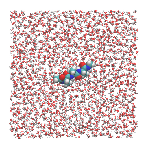
In this tutorial, we will simulate (Ala)3 in water. First, we build a system using VMD/PSFGEN from a PDB file of the (Ala)3 and the CHARMM topology file. This scheme is identical to Steps 1, 3, and 4 in Tutorial 2.3. The peptide is solvated in a water box (50.2 Å × 50.2 Å × 50.2 Å). We obtain wbox.pdb and wbox.psf as input files for GENESIS. The total number of atoms in this system is about 12,000.
# Change directory for the system setup
$ cd 1_setup
$ ls
1_oripdb  2_psfgen  3_solvate

# Download the PDB file
$ cd 1_oripdb
$ ln -s ../../../../Data/PDB/ala3.pdb ./
$ ls
ala3.pdb

# Make PDB and PSF files
$ cd ../2_psfgen
$ vmd -dispdev text -e build.tcl > log
$ ls
build.tcl  log  proa.pdb  proa.psf

# Solvate the peptide in water
$ cd ../3_solvate
$ vmd -dispdev text -e build.tcl > log
$ ls
$ build.tcl  log  wbox.log  wbox.pdb  wbox.psf

# View the initial structure
$ vmd wbox.pdb -psf wbox.psf
2. Minimization
In the previous tutorial (Tutorial 3.1), we just performed MD simulation. However, in most cases, energy minimization must be performed before MD simulations to remove atomic clash in the initial structure. In general, energy minimization is a method of minimizing the potential energy of the system by simply moving the atoms gradually in the direction of the force acting on them. One of the most popular methods is the steepest descent method, which is introduced in GENESIS. Let’s change the directory to perform energy minimization and look at the GENESIS control file.
# Change directory for the energy minimization
$ cd ../../2_minimize

# View the control file
$ less INP
In the [MINIMIZE] section of the control file, we specify the method to be used in the energy minimization. Here, the steepest descent (SD) method is used to perform a 2,000-steps energy minimization. Since the target system has a periodic boundary condition (PBC), we set type = PBC in the [BOUNDARY] section and also set the initial box size with box_size = 50.2.
Since the system has a periodic boundary condition and the total charge is zero, the Ewald method can be used. The particle mesh Ewald method (PME) is employed to calculate long-range interactions [2] and is specified by electrostatic = PME in the [ENERGY] section. A cutoff distance of 12.0 Å is used for non-bonded interactions and a switching distance of 10.0 Å is used for van der Waals interactions. This combination of switch and cutoff distances has recently been recommended for MD simulations using the CHARMM C36 force field and explicit solvent. In the same section, you can find “contact_check = YES“, which is usually essential to avoid instabilities in the early stages of the energy minimization (for details, see the User manual).
The top_all36_prot.rtf and par_all36m_prot.prm specified in the [INPUT] section contain only the force field parameters for amino acids. However, information on water and ions is not included in these files. Therefore, another file (toppar_water_ions.str) containing topology and parameters for water and ions is further passed to the [INPUT] section. In the [OUTPUT] section, dcdfile and rstfile are specified. Here, the rstfile is a “restart file” and contains the coordinates of the atoms at the final step of the energy minimization. This file will be used as the input file for the subsequent MD simulation.
[INPUT]
topfile = ../toppar/top_all36_prot.rtf     # topology file
parfile = ../toppar/par_all36m_prot.prm    # parameter file
strfile = ../toppar/toppar_water_ions.str  # stream file
psffile = ../1_setup/3_solvate/wbox.psf    # protein structure file
pdbfile = ../1_setup/3_solvate/wbox.pdb    # PDB file

[OUTPUT]
dcdfile = min.dcd          # DCD trajectory file
rstfile = min.rst          # restart file

[ENERGY]
forcefield       = CHARMM  # [CHARMM]
electrostatic    = PME     # [PME]
switchdist       = 10.0    # switch distance
cutoffdist       = 12.0    # cutoff distance
pairlistdist     = 13.5    # pair-list distance
vdw_force_switch = YES     # force switch option for van der Waals
contact_check    = YES     # check atomic clash

[MINIMIZE]
method           = SD      # [SD]
nsteps           = 2000    # number of minimization steps
eneout_period    =   50    # energy output period
crdout_period    =   50    # coordinates output period
rstout_period    = 2000    # restart output period
nbupdate_period  =   10    # nonbond update period

[BOUNDARY]
type             = PBC     # [PBC]
box_size_x       = 50.2    # box size (x) in [PBC]
box_size_y       = 50.2    # box size (y) in [PBC]
box_size_z       = 50.2    # box size (z) in [PBC]
Let’s run energy minimization using spdyn. The following command uses 4 MPI processors and 4 OpenMP threads, i.e., a total of 16 CPU cores. The actual number of availavle CPU cores depends on the user’s computer environment and should be set to an appropriate value by the user (see the Usage page for details). It takes ~30 seconds to complete the calculation. After the calculation is finished, check the trajectory in VMD. You can see that the atoms have moved a little and that the clash between atoms seems to be removed.
# Run energy minimization (it takes ~30 seconds)
$ export OMP_NUM_THREADS=4
$ mpirun -np 4 ../bin/spdyn INP > log

# View the trajectory using VMD
$ vmd ../1_setup/3_solvate/wbox.pdb -dcd min.dcd
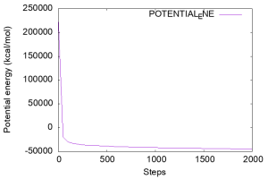
Let’s check the potential energy, which is written in the 3rd column of the INFO: line of the log file. Below is an example of a command to plot the time course of the potential energy using Gnuplot. In the previous tutorial (see Sub-section 3.1 of Tutorial 3.1), we ran the grep command before gnuplot to create “energy.log“. The grep command can be placed directly inside the gnuplot command. In the figure you can see that the potential energy is well decreased during the minimization.
# Check the potential energy change
$ gnuplot
gnuplot> set key autotitle columnhead
gnuplot> set xlabel "Steps"
gnuplot> set ylabel "Potential energy (kcal/mol)"
gnuplot> plot '< grep "INFO:" log' u 2:3 with lines
The root-mean-square gradient (RMSG) is another criteria to validate the energy minimization, which is written in the 4th column of the log file. Let’s plot the RMSG as well.
3. Equilibration
The goal of this tutorial is to perform an MD simulation of the peptide in the NPT ensemble at T = 300 K and P = 1 atm. Of course, you can start MD simulations in the NPT ensemble from the beginning. However, this is generally not recommended because the initial structure constructed in 1_setup is artificial, which may affect the accuracy and stability of the initial stage of the MD simulation. Specifically, the density of water around the peptide in the initial structure may deviate from the experimental or ideal value at T = 300 K and P = 1 atm. If an MD simulation is performed for such a system immediately after energy minimization, the simulation may become unstable due to the strong forces generated on the atoms to control the temperature and pressure. Such strong forces may also destroy the protein structure. Therefore, it is usually necessary to equilibrate the system gradually. In this tutorial, we will introduce a general scheme for the equilibration.
Let’s change the directory for equalization. This directory contains three control files (INP1–3). We will use spdyn to run INP1 through INP3.
# Change directory for the equilibration
$ cd ../3_equilibrate
$ ls
INP1  INP2  INP3
Step1. NVT-MD with positional restraint
In Step 1, a short MD simulation is performed in the NVT ensemble using INP1, where the position of the peptide is fixed usig a positional restraint. That is, only water molecules are equilibrated. The NVT ensemble allows the system to equilibrate more moderately than the NPT ensemble.
The following is an important part of the control file. We carry out a 50-ps MD simulation at T = 300 K. The equations of motion are integrated with a time step of 2 fs with the velocity Verlet algorithm, and the bond lengths involving hydrogen atoms are constrained using the SHAKE/RATTLE [3,4] and SETTLE algorithms [5]. Temperature is controlled with the Bussi thermostat [6]. The [ENERGY] section is the same as in the previous energy minimization. In the [BOUNDARY] section, the box size is not specified, since the atomic coordinates and box size are taken over from the restart file (min.rst).
Positional restraints are specified using the [SELECTION] and [RESTRAINTS] sections. In the [SELECTION] section we select the heavy atom of the peptide by “sid:PROA and heavy” (sid means segment index). As you can see in wbox.pdb, this peptide has a segment name “PROA“. In the [RESTRAINTS] section, we turn on the positional constraint (POSI) and set the force constant of the restraint function to 1 kcal/mol/Å2. The reference coordinates of the positional restraint are given in the reffile in the [INPUT] section.
[INPUT]
:
pdbfile = ../1_setup/3_solvate/wbox.pdb    # PDB file
reffile = ../1_setup/3_solvate/wbox.pdb    # reference PDB file for restraint
rstfile = ../2_minimize/min.rst            # restart file

[DYNAMICS]
integrator       =   VVER   # [VVER]
nsteps           =  25000   # number of MD steps
timestep         =  0.002   # timestep (ps)
eneout_period    =    500   # energy output period
crdout_period    =    500   # coordinates output period
rstout_period    =  25000   # restart output period
nbupdate_period  =     10   # nonbond update period

[ENSEMBLE]
ensemble         = NVT      # [NVE,NVT,NPT,NPAT,NPgT]
tpcontrol        = BUSSI    # [NO,BERENDSEN,BUSSI,NHC]
temperature      = 300      # initial and target temperature (K)

[BOUNDARY]
type             = PBC      # [PBC]

[SELECTION]
group1           = sid:PROA and heavy  # restraint group 1

[RESTRAINTS]
nfunctions       = 1        # number of restraint functions
function1        = POSI     # POSI: Positional restraint is employed
direction1       = ALL      # ALL: x,y,z-coordinates are restrained
constant1        = 1.0      # force constant (kcal/mol/A^2)
select_index1    = 1        # restrained groups
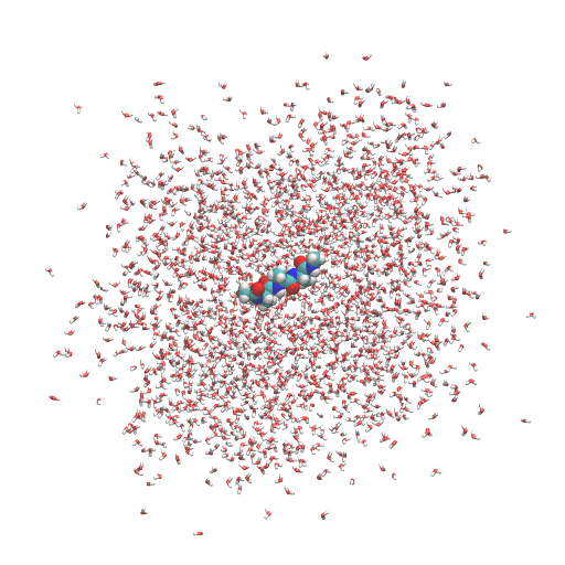
Let’s run spdyn with INP1 and watch the resulting trajectory in VMD. We can see that the peptide is fixed at the center of the system due to the positional restraint. We also see that the water molecules are spread out from the simulation box. This is actually not a problem because we are considering a periodic boundary condition. Water molecules outside the box are located in the “image” cells.
# Run the equilibration MD step1 (it takes ~5 minutes)
$ mpirun -np 4 ../bin/spdyn INP1 > log1

# View the trajectory using VMD
$ vmd ../1_setup/3_solvate/wbox.pdb -dcd eq1.dcd
If you want to wrap all molecules into the unit cell, the following VMD command is useful:
# View the trajectory using VMD (all molecules are wrapped into the unit cell)
$ vmd ../1_setup/3_solvate/wbox.pdb -dcd eq1.dcd
vmd > pbc wrap -compound fragment -center origin -all
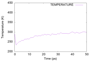
Using gnuplot, let’s look at the time course of the temperature (column 17 of the log file). We can see that the temperature was very high (~450 K) in the early stages of the simulation. This is probably due to the strong forces generated in the artificial initial structure, which generated fast velocities for many water molecules. The temperature then suddenly dropped to 250 K, but gradually increased to 300 K during 50 ps, suggesting that the water molecules had nearly equilibrated.
Step2. NPT-MD with positional restraint
In Step 2, the ensemble is switched to NPT to adjust the box size. In the [ENSENBLE] section, we specify “ensemble = NPT“. The target pressure P = 1 atm is also set in the same section. The other sections and parameters are the same as in Step 1. Here, we run a 50-ps MD simulation at T = 300 K and P = 1 atm using the Bussi thermostat and barostat [6,7]. Again, the equations of motion are integrated with a time step of 2 fs with the velocity Verlet algorithm, and the SHAKE/RATTLE and SETTLE algorithms are employed for bond constraints. Positional constraints are still applied to the heavy atoms of the peptide. By specifying the restart file obtained in Step 1 in [INPUT], the atomic coordinates and velocities at the last step in Step 1 are used as the initial coordinates and velocities in this run.
[ENSEMBLE]
ensemble         = NPT      # [NVE,NVT,NPT,NPAT,NPgT]
tpcontrol        = BUSSI    # [NO,BERENDSEN,BUSSI,NHC]
temperature      = 300      # initial and target temperature (K)
pressure         = 1.0      # target pressure (atm)
Let’s run spdyn with INP2 and watch the resulting trajectory in VMD.
# Run the equilibration MD step2 (it takes ~5 minutes)
$ mpirun -np 4 ../bin/spdyn INP2 > log2

# View the trajectory using VMD
$ vmd ../1_setup/3_solvate/wbox.pdb -dcd eq2.dcd
vmd > pbc wrap -compound fragment -center origin -all
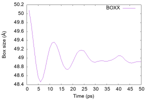
Let’s check the time course of the box size (column 19 of the log file), which should vary with the NPT ensemble. We see that the box shrinks rapidly within 5 ps and oscillates after 10 ps, implying that the density of water was regulated.
Let’s plot the pressure as well.
Step3. Pre-production run with restraint
In Steps 1 and 2, we used the velocity Verlet integrator (VVER) with a time step of 2 fs. This is because we want to carefully equilibrate the system. However, if we run the production calculations with 2fs VVER, that is the “old fashioned way”. For production calculations, we would like to use the RESPA integrator (VRES) [8], i.e., a “more advanced method,” with a time step of 2.5 fs to extend the simulation time. Since we need to switch from 2 fs VVER to 2.5 fs RESPA, in Step 3 we equilibrate the system again using RESPA. We perform a 50-ps MD simulation at T = 300 K and P = 1 atm using the Bussi thermostat and barostat. Positional restraints are applied to the heavy atoms of the peptide. In the RESPA scheme, the PME calculation is performed every 2 steps and the thermostat and barostat momentum are updated every 10 steps. In addition, group_tp is turned on in the [ENSEMBLE] section, which is requred to employ the VRES integrator.
[DYNAMICS]
integrator        =   VRES  # [VRES]
nsteps            =  20000  # number of MD steps (50ps)
timestep          = 0.0025  # timestep (2.5fs)
eneout_period     =    400  # energy output period (1ps)
crdout_period     =    400  # coordinates output period (1ps)
rstout_period     =  20000  # restart output period
nbupdate_period   =     10  # nonbond update period
elec_long_period  =      2  # period of reciprocal space calculation
thermostat_period =     10  # period of thermostat update
barostat_period   =     10  # period of barostat update

[ENSEMBLE]
ensemble          =    NPT  # [NVE,NVT,NPT,NPAT,NPgT]
tpcontrol         =  BUSSI  # [NO,BERENDSEN,BUSSI,NHC]
temperature       =    300  # initial and target temperature (K)
pressure          =    1.0  # target pressure (atm)
group_tp          =    YES  # usage of group tempeature and pressure
Now let’s run spdyn with INP3. To compare the computational times, let’s use the same number of CPU cores as in Step 2.
# Run the equilibration MD step3
$ mpirun -np 4 ../bin/spdyn INP3 > log3
We can see that the elapsed time in Step 3 is much shorter (~1.5x) than in Step 2, even though the same 50 ps MD simulation was performed in Step 3. The resulting restart file (eq3.rst) will be used in the subsequent production run.
# Compare the computational time between Step2 and Step3
$ grep "dynamics      =" log2 log3
log2:    dynamics      =     343.291
log3:    dynamics      =     227.322
In general, it is difficult to determine when to stop equilibration. In this tutorial, we stopped equilibration at 50 ps in each step because the temperature reached the target value in Step 1 and the box size showed stable oscillations in Step 2. The appropriate time should depend on the system. Larger systems or more complex systems such as membrane proteins usually require longer equilibration time (e.g., 10 ns or longer).
4. Production
Finally, the production runs are carried out. The simulation conditions are the same as in the previous equilibration step 3, but with the positional restraints turned off. We will perform a 500-ps MD simulation in the NPT ensemble at T = 300 K and P = 1 atm. In the directory, you will find 5 control files.
# Change directory for production run
$ cd ../4_production
$ ls
INP1  INP2  INP3  INP4  INP5
Now, let’s run spdyn sequentially for INP1 through INP5, each of which is corresponding to a 100 ps MD run. We will obtain 500-ps MD trajectories in total.
# Production run for   0-100 ps (restart from eq3.rst)
$ mpirun -np 4 ../bin/spdyn INP1 > log1

# Production run for 100-200 ps (restart from md1.rst)
$ mpirun -np 4 ../bin/spdyn INP2 > log2

# Production run for 200-300 ps (restart from md2.rst)
$ mpirun -np 4 ../bin/spdyn INP3 > log3

# Production run for 300-400 ps (restart from md3.rst)
$ mpirun -np 4 ../bin/spdyn INP4 > log4

# Production run for 400-500 ps (restart from md4.rst)
$ mpirun -np 4 ../bin/spdyn INP5 > log5
Of course, it is possible to set the MD step to 200,000 and perform 500 ps MD with a single control file only. But remember that in most cases “short multiple consecutive runs” are substantially more convenient than a “long single run”. The purpose is primarily for quick recovery against computer accidents, such as a power failure, or to finish one job in a limited time.
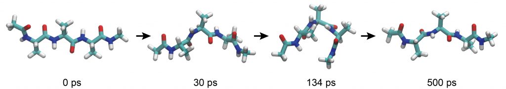
We obtain log1, md1.dcd, md1.rst from INP1 for the first 100 ps, …, and log5, md5.dcd, md5.rst from INP5 for the last 100-ps. Let’s take a look at the trajectory using VMD. You can load all trajectory files at the same time with the following command. You can see that the peptide fluctuates and the conformation changes from time to time.
# Check the output files
$ ls
INP1  INP3  INP5  log2  log4  md1.dcd  md2.dcd  md3.dcd  md4.dcd  md5.dcd
INP2  INP4  log1  log3  log5  md1.rst  md2.rst  md3.rst  md4.rst  md5.rst

# View the 500-ps MD trajectories using VMD
$ vmd ../1_setup/3_solvate/wbox.pdb -dcd md1.dcd md2.dcd md3.dcd md4.dcd md5.dcd

# Read the DCD files sequentially from md1.dcd to md5.dcd
$ vmd ../1_setup/3_solvate/wbox.pdb -dcd md{1..5}.dcd
5. Analysis
Now, there are five log files for energy trajectories and five DCD files for the coordinates trajectories. Here, we will learn how to deal with these multiple log files and multiple DCD files.
# Change directory for trajectory analysis
$ cd ../5_analysis
$ ls
1_energy  2_distance
5.1 Energy
First, let’s analyze the time course of the temperature over 500 ps. The temperature is shown in the 16th column of the log1-5 files. We pick up the “INFO:” lines from log1 with the grep command, but exclude the first line (header information) with “tail -n +2“. The result is written to “energy.log“. Next, run the same command for log2 with “>>” for additional writing of the result to “energy.log“. This is repeated until log5. Finally, the combined log data is obtained.
# Combine all log data
$ cd 1_energy

# Combine all log data
$ grep "INFO:" ../../4_production/log1 | tail -n +2 >  energy.log
$ grep "INFO:" ../../4_production/log2 | tail -n +2 >> energy.log
$ grep "INFO:" ../../4_production/log3 | tail -n +2 >> energy.log
$ grep "INFO:" ../../4_production/log4 | tail -n +2 >> energy.log
$ grep "INFO:" ../../4_production/log5 | tail -n +2 >> energy.log
Let’s plot the time course of the temperature using gnuplot. In the previous tutorial (Tutorial 3.1), we used the 3rd column on the X axis, which simply corresponds to the simulation time. However, in this combined log file, the 3rd column can no longer be used because the time has been reset to 0 ps after the restart (see the first step in log2). Therefore, we use the “0th” column instead, which corresponds to the “line number” for the plot. Now, in energy.log there are 1,000 lines. We can convert the line number to time by dividing the 0th column by 2, which is specified by “($0/2)” in the gnuplot command:
# Plot the temperature change
$ gnuplot
gnuplot> unset key
gnuplot> set xlabel "Time (ps)"
gnuplot> set ylabel "Temperature (K)"
gnuplot> plot 'energy.log' u ($0/2):16 with lines
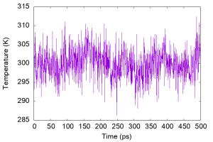
We can see that the temperature fluctuates around a certain value, and the average temperature is actually close to the target temperature.
# Compute the averaged temperature over 500 ps
$ awk '{sum+=$16} END {print sum/NR}' energy.log
299.993
5.2 Distance
Next, let us analyze the distance between the selected atoms in the peptide. Here, we select the “OY” atom at the N-terminus and the “HNT” atom at the C-terminus.
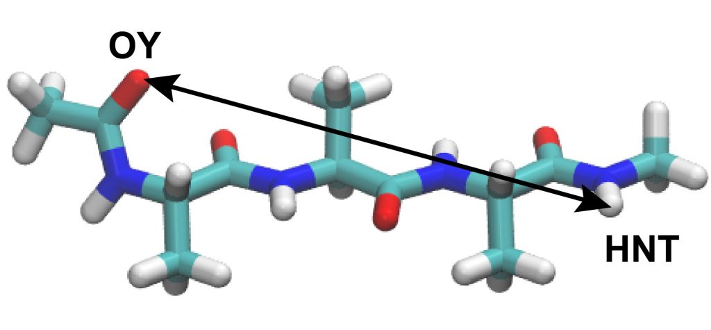
These two atoms should form a hydrogen bond if the peptide forms an α-helix conformation. The control file for the analysis is already included in the directory. Here, we will use the “trj_analysis” tool as in Tutorial 3.1, subsection 3.2.
$ cd ../2_distance
$ ls
INP

# View the control file
$ less INP
In the [TRAJECTORY] section, we set md1.dcd, md2.dcd. …, and md5.dcd. Since we have carried out 40,000-steps MD simulation with crdout_period = 200 in each production run, we specify md_step1 = 40000 and mdout_period1 = 200. Since we want to analyze all snapshots in each run, ana_period1 is set to be equal to mdout_period1. Here, “repeat1 = 5” means that the analysis using “md_step1 = 40000“, “mdout_perioud1 = 200“, and “ana_period1 = 200” is repeated 5 times for the trajfile1-5. In the [OPTION] section, we select the atoms to be analyzed.
[INPUT]
psffile = ../../1_setup/3_solvate/wbox.psf  # protein structure file
reffile = ../../1_setup/3_solvate/wbox.pdb  # PDB file

[OUTPUT]
disfile = output.dis                        # distance file

[TRAJECTORY]
trjfile1      = ../../4_production/md1.dcd  # trajectory file
trjfile2      = ../../4_production/md2.dcd  # trajectory file
trjfile3      = ../../4_production/md3.dcd  # trajectory file
trjfile4      = ../../4_production/md4.dcd  # trajectory file
trjfile5      = ../../4_production/md5.dcd  # trajectory file
md_step1      = 40000                       # number of MD steps
mdout_period1 = 200                         # MD output period
ana_period1   = 200                         # analysis period
repeat1       = 5
trj_format    = DCD               # (PDB/DCD)
trj_type      = COOR+BOX          # (COOR/COOR+BOX)
trj_natom     = 0                 # (0:uses reference PDB atom count)

[OPTION]
distance1     = PROA:1:ALA:OY   PROA:3:ALA:HNT
Let’s run trj_analysis with this control file. You will obtain “output.dis“, in which the results of the distance calculation is output in the 2nd column.
# Analyze the time courses of dihedral angle PHI and PSI
$ ../../bin/trj_analysis INP > log
$ ls
INP  log  output.dis

# Time courses of the dihedral angles phi and psi
$ gnuplot
gnuplot> set encoding iso
gnuplot> set xlabel 'Time (ps)'
gnuplot> set ylabel 'Distance (\305)'
gnuplot> plot 'output.dis' u ($1/2):2 t "OY-HNT distance" with lines
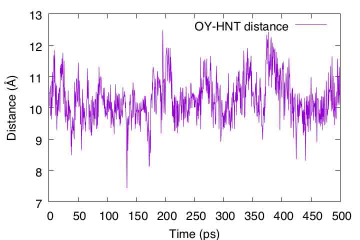
If the peptide formed an α-helix, the distance should be closer to 2 Å. However, the distance actually fluctuated around 10 Å. As also seen in VMD, the peptide tends to form extended conformations rather than α-helixes in the aqueous environment.
References
- J. Huang et al., Nat. Methods, 14, 71-73 (2017).
- T. Darden et al., J. Chem. Phys., 98, 10089-10092 (1993).
- J. P. Ryckaert et al., J. Comput. Phys., 23, 327-341 (1977).
- H. Andersen, J. Comp. Phys., 52, 24-34 (1983).
- S. Miyamoto and P. A. Kollman, J. Comput. Chem., 13, 952-962 (1992).
- G. Bussi et al., J. Chem. Phys., 126, 014101 (2007).
- G. Bussi et al., J. Chem. Phys., 130, 074101 (2009).
- M. Tuckerman et al., J. Chem. Phys., 97, 1990-2001 (1992).
Written by Takaharu Mori@RIKEN Theoretical molecular science laboratory
April 26, 2022