3.1 MD simulation of alanine-dipeptide in the gas-phase
Contents
Preparation
First, let’s download the tutorial file (tutorial19-3.1.zip). This tutorial consists of three steps: 1) system setup, 2) MD simulation, and 3) trajectory analysis. GENESIS control file in each step is already included in the download file. To use the CHARMM36m force field parameters [1], let’s create a symbolic link to the CHARMM toppar directory (see Tutorial 2.2), and in addition, create a symbolic link to the GENESIS bin directory (see Tutorial 1.1).
# Download the tutorial file
$ cd ~/GENESIS_Tutorials-2019/Works
$ mv ~/Downloads/tutorial19-3.1.zip ./
$ unzip tutorial19-3.1.zip

# Clean up the directory
$ mv tutorial19-3.1.zip TRASH

# Update the README file
$ echo "tutorial-3.1: MD simulation of alanine-dipeptide in gas" >> README

# Check out the contents in Tutorial 3.1
$ cd tutorial-3.1
$ ln -s ../../Data/Parameters/toppar_c36_jul21 ./toppar
$ ln -s ../../Programs/genesis-1.7.1/bin ./bin
$ ls
1_setup  2_runmd  3_trjana  bin  toppar
1. Setup
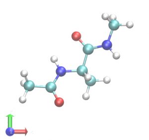
In this tutorial, we will simulate alanine-dipeptide in the gas phase, i.e., without solvent molecules. First, we build a system using VMD/PSFGEN from a PDB file of the alanine-dipeptide. The scheme is the same as in Steps1 and 3 of Tutorial 2.3. We obtain proa.pdb and proa.psf as the input files for GENESIS. The peptide has one alanine residue, with the N- and C-termini capped by acetyl (CH3CO-) and N-methyl (-NHCH3) groups, respectively. This structure has already been optimized by energy minimization and there are no clashes between atoms. Therefore, MD simulations can be started immediately. Note that in most cases, energy minimization is required before MD simulation (e.g. Tutorials 3.2 and 3.3).
# Change directory for the system setup
$ cd 1_setup
$ ls
1_oripdb  2_psfgen

# Step1: Make a symbolic link to the original PDB file
$ cd 1_oripdb
$ ln -s ../../../../Data/PDB/ala2.pdb ./

# Step2: Make PDB and PSF files
$ cd ../2_psfgen
$ ls
build.tcl

$ vmd -dispdev text -e build.tcl > log
$ ls
ala2.pdb  build.tcl  log  proa.pdb  proa.psf

# View the initial structure
$ vmd proa.pdb -psf proa.psf
2. MD simulation
To run the MD simulation of this peptide, change the directory to 2_runmd. This directory already contains the GENESIS control file. Let’s look at it and check the simulation conditions.
# Change directory to run MD simulation
$ cd ../../2_runmd
$ ls
INP

# View the control file
$ less INP
In the control file, the [INPUT] section specifies the topology and parameter files for the CHARMMC36m force field. The psf and pdb files created in Step1 are also specified. In the [OUTPUT] section, the filename of the coordinates trajectory data obtained from the MD simulation is specified with “dcdfile“. Since the system is in the gas phase, non-bonded interactions are calculated with the usual cutoff scheme (electrostatic = CUTOFF) instead of the Ewald method. Therefore, we need to use as long a cutoff distance as possible. Here we calculate the potential energy with the cutoff distance of 49 Å, as specified in the [ENERGY] section.
We use the velocity Verlet integrator (VVER) with a time step of 2 fs ([DYNAMICS]), where the SHAKE [2] and RATTLE algorithms [3] are used for constraining the bond length involving hydrogen ([CONSTRAINTS]). The energy and coordinates are output every 500 steps ([DYNAMICS]). We use the Bussi thermostat [4] to keep the temperature constant at 298.15 K ([ENSEMBLE]). Since the system is the gas-phase, we do not use the periodic boundary condition, namely, boundary type is set to “NOBC” (no boundary condition) ([BOUNDARY]). We carry out a 1-ns MD simulation (nsteps = 500000).
[INPUT]
topfile = ../toppar/top_all36_prot.rtf   # topology file
parfile = ../toppar/par_all36m_prot.prm  # parameter file
psffile = ../1_setup/2_psfgen/proa.psf   # protein structure file
pdbfile = ../1_setup/2_psfgen/proa.pdb   # PDB file

[OUTPUT]
dcdfile = md.dcd             # Coordinates trajectory file

[ENERGY]
forcefield       = CHARMM    # CHARMM force field
electrostatic    = CUTOFF    # cutoff scheme is used
switchdist       =   48.0    # switch distance
cutoffdist       =   49.0    # cutoff distance
pairlistdist     =   50.0    # pair-list distance

[DYNAMICS]
integrator       =   VVER    # velocity Verlet
nsteps           = 500000    # number of MD steps
timestep         =  0.002    # timestep (ps)
eneout_period    =    500    # energy output period
crdout_period    =    500    # coordinates output period
stoptr_period    =     10    # remove translational and rotational motions

[CONSTRAINTS]
rigid_bond       = YES       # use SHAKE/RATTLE

[ENSEMBLE]
ensemble         = NVT       # Canonical ensemble
tpcontrol        = BUSSI     # Bussi thermostat
temperature      = 298.15    # initial and target temperature (K)

[BOUNDARY]
type             = NOBC      # non-periodic system
Now let’s run GENESIS. ATDYN is more suitable than SPDYN for this simulation because the peptide is very small and the system is non-periodic. Here we specify one OpenMP thread and use only one CPU core for the calculation (see the Usage page for details). The simulation takes approximately 20 seconds. Specifying “> log” on the command line will write the output message to log (this procedure is called “Redirection“). if “> log” is omitted, the message will be displayed in the terminal window.
# Run the MD simulation (it takes ~20 seconds)
$ export OMP_NUM_THREADS=1
$ ../bin/atdyn INP > log
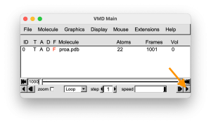
After the simulation is finished, we can obtain md.dcd and log as the “coordinates” and “energy” trajectory of the system, respectively. Visualize the coordinates trajectory with VMD. Press the “Play” button in the VMD main window. You can see that the atoms of the peptide are moving fast.
# Check the output files
$ ls
INP  log  md.dcd

# View the MD trajectory using VMD
$ vmd ../1_setup/2_psfgen/proa.pdb -dcd md.dcd
The resulting DCD file is a binary file, not a text file. So, even if you use the less command for the dcd file, its contents cannot be visually confirmed by human eyes. In Tutorial 4.1, you will learn how to handle DCD files.
Also, let’s take a look at the log file with the less command.
# View the log file
$ less log
In the middle of the log file, there are many lines beginning with “INFO:“. In these lines, system information at each step is displayed, where STEP is the number of MD steps, TIME is the simulation time (in picoseconds), TOTAL_ENE is the sum of the potential energy (POTENTIAL_ENE) and kinetic energy (KINETIC_ENE), RMSG is the gradient of the potential energy averaged over all atoms (root-mean-square gradient). The components of the potential energy of the CHARMM force field are then displayed (bond, angle, Urey-Bradley, dihedral angle, improper torsion angle, CMAP, van der Waals, Coulomb). TEMPERATURE is the system temperature, which is calculated from the kinetic energy and velocities by Ke = 1/2Σmivi2 = 3/2NkBT. The unit of the energy is kcal/mol, and temperature is Kelvin.
:
INFO:       STEP            TIME       TOTAL_ENE   POTENTIAL_ENE     KINETIC_ENE
            RMSG            BOND           ANGLE    UREY-BRADLEY        DIHEDRAL
        IMPROPER            CMAP         VDWAALS           ELECT     TEMPERATURE
          VOLUME
 --------------- --------------- --------------- --------------- ---------------
INFO:          0          0.0000         -6.0756        -16.3544         10.2788
          0.7599          0.3534          0.6844          0.1145          3.5537
          0.0216         -1.2625         -1.0729        -18.7464        215.5215
          0.0000

INFO:        500          1.0000         -3.6016        -10.1971          6.5955
         10.0918          2.4181          4.5486          0.4363          4.1692
          0.1899         -1.2175         -0.8483        -19.8936        138.2915
          0.0000
:
Please note that your detailed results may differ from the above results. The main reason is that the initial velocities of atoms vary depending on the random number seed, and the seed is automatically determined according to the time the program is executed, unless you specify a seed value. If you want to fix the initial seed value, set “iseed” explicitly in the [DYNAMICS] section (see the User manual).
VOLUME is the volume of the system. In this case, zero is output, since we employed the gas-phase. If periodic system is simulated as in Tutorial 3.2, the volume of the simulation box is displayed in this column.
At the end of the log file, detailed computation times for this simulation are displayed, with timers for energy calculation, integrator, pair list making, and so on. “setup” is the time taken to start the MD simulation, including loading the input file and initial memory allocation, and “dynamics” represents the time for pure MD simulation, excluding initial setup. It can be seen that the most time consuming part is the non-bonded energy calculation (van der Waals and Coulomb terms).
# View the last 100 lines of log
$ tail -100 log
Output_Time> Averaged timer profile (Min, Max)
  total time      =      13.266
    setup         =       0.133
    dynamics      =      13.133
      energy      =      11.084
      integrator  =       1.730
      pairlist    =       0.140 (       0.140,       0.140)
  energy
    bond          =       0.279 (       0.279,       0.279)
    angle         =       2.560 (       2.560,       2.560)
    dihedral      =       3.069 (       3.069,       3.069)
    nonbond       =       4.193 (       4.193,       4.193)
:
  integrator
    constraint    =       1.234 (       1.234,       1.234)
:
3. Trajectory analysis
Now let’s analyze the energy and conformational changes of the peptide from the trajectory data.
# Change directory for trajectory analysis
$ cd ../3_trjana/
$ ls
1_energy  2_dihedral
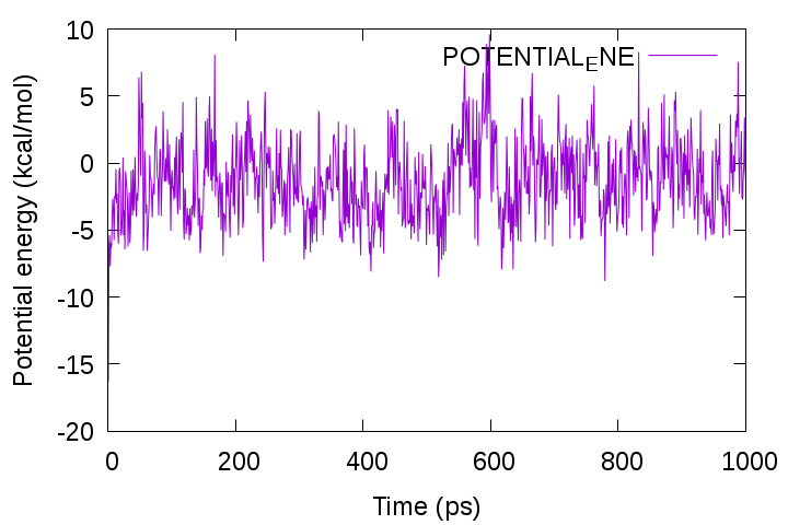
3.1 Energy
Let’s plot the time course of the potential energy using Gnuplot. First, pick up the lines containing “INFO:” from the log file with the grep command and write them into a new file “energy.log“. Then, plot the 5th column, which corresponds to the total potential energy. You can see that the energy fluctuates around a certain value.
# Change directory for trajectory analysis
$ cd 1_energy

# Select lines that contain "INFO:" using the "grep" command
$ grep "INFO:" ../../2_runmd/log > energy.log
$ less energy.log

# View the time courses of energy using gnuplot
$ gnuplot
gnuplot> set key autotitle columnhead
gnuplot> set xlabel "Time (ps)"
gnuplot> set ylabel "Potential energy (kcal/mol)"
gnuplot> plot 'energy.log' using 3:5 with lines
If you want to pick up the columns of time (3rd column) and total potential energy (5th column) at the same time, the awk command is useful:
# Pick up the 3rd and 5th columns
$ awk '{print $3, $5}' energy.log > potential_ene.log
$ less potential_ene.log
Now let’s calculate the averaged potential energy from potential_ene.log. The averaged value for each column can be quickly calculated with the awk command. The following is an example, analyzing the 2nd column of potential_ene.log. This file consists of 1,002 lines, and the first two lines (header information and initial step energy) are skipped in the analysis.
# Compute the averaged potential energy using the tail and awk commands
$ tail -1000 potential_ene.log > tmp
$ awk '{sum+=$2} END {print sum/NR}' tmp
-1.30413

# The above two commands can be combined with the pipeline "|"
$ tail -1000 potential_ene.log | awk '{sum+=$2} END {print sum/NR}'
-1.30413
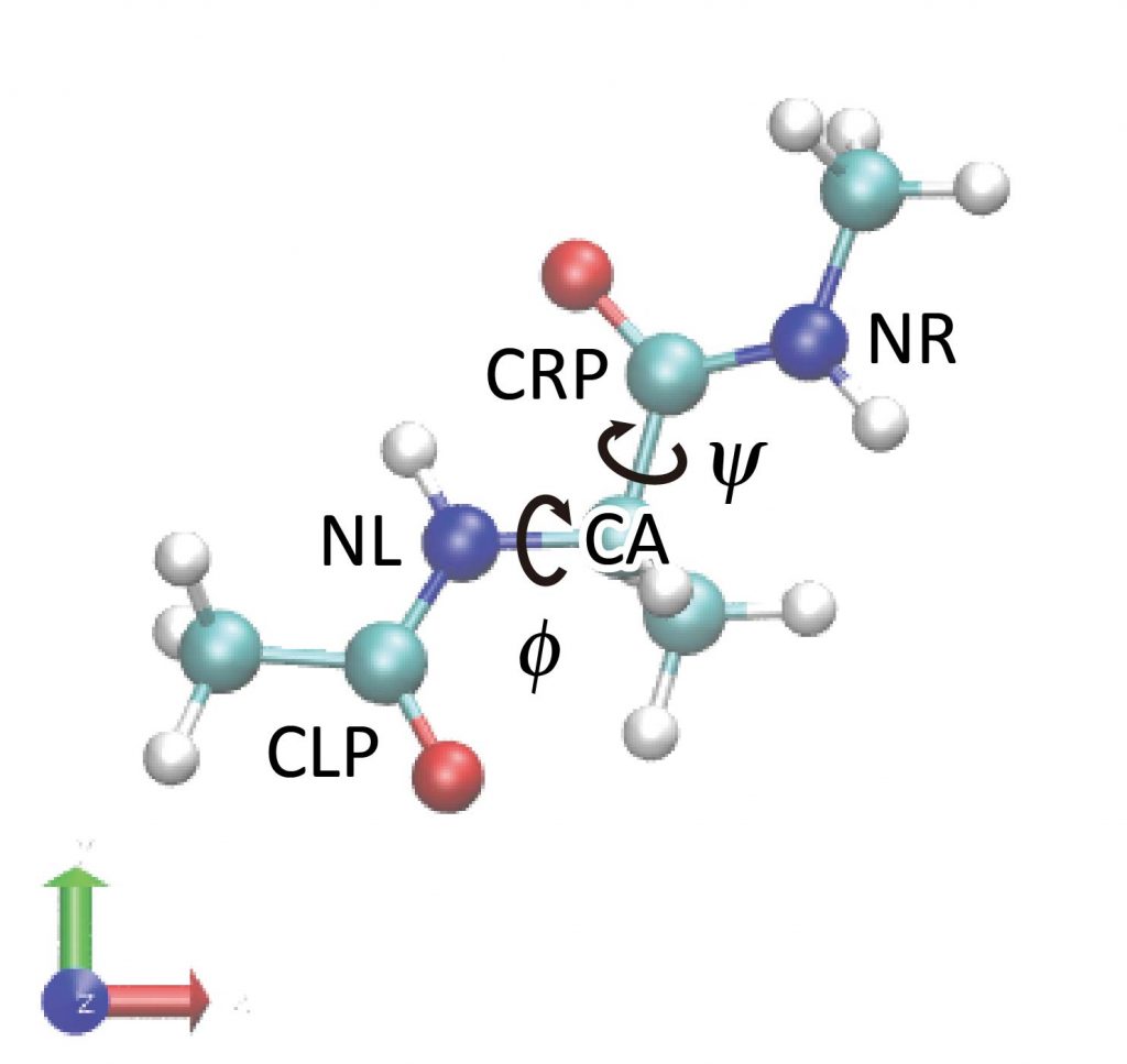
3.2 Dihedral angle
We analyze the conformational changes of the peptide using the GENESIS trajectory analysis tool. The peptide has two major variables that can describe its conformation: φ and ψ (backbone dihedral angle). φ is the dihedral angle of the C-N-Cα-C atoms and ψ is the dihedral angle of the N-Cα-C-N atoms. The trj_analysis tool is used to analyze these dihedral angles, whose control file is shown below.
# Change directory for the analysis of dihedral angles
$ cd ../2_dihedral
$ ls
INP

# View the control file (see below)
$ less INP
We specify the input and output files in the [INPUT] and [OUTPUT] sections. In the [TRAJECTORY] section, we specify the number of MD steps and coordinates output period corresponding to the DCD file to be analyzed and the nsteps and crdout_period in the ATDYN control file, respectively (for details on [TRAJECTORY], see the FAQ). The [OPTION] section sets the list of atoms to be used in the dihedral angle calculation. These atom names should be written carefully by looking at the molecular structure in VMD or by checking the PDB file. Here, the syntax for atom selection is [segnemt_name]:[residue_id]:[residue_name]:[atom_name]. In particular, PROA:1:ALAD:CA means the Cα atom of ALAD1 in segment:PROA.
We specify the input and output files in the [INPUT] and [OUTPUT] sections. In the [TRAJECTORY] section, we specify the DCD file to be analyzed, and also total number of MD steps (md_step) and MD output period (mdout_period), each of which is corresponding to nsteps and crdout_period in the control file of ATDYN, respectively (For more detailed description of the [TRAJECTORY] section, see Appendix). In the [OPTION] section, we set atom lists to be used for the dihedral angle calculation. These atom names should be written carefully by looking at the molecular structure in VMD or by checking the PDB file. Here, the syntax of the atom selection is [segnemt_name]:[residue_id]:[residue_name]:[atom_name]. In particular, PROA:1:ALAD:CA means the Cα atom of ALAD1 in segment:PROA.
[INPUT]
psffile       = ../../1_setup/2_psfgen/proa.psf  # protein structure file
reffile       = ../../1_setup/2_psfgen/proa.pdb  # PDB file

[OUTPUT]
torfile       = output.tor              # torsion file

[TRAJECTORY]
trjfile1      = ../../2_runmd/md.dcd    # trajectory file
md_step1      = 500000                  # number of MD steps
mdout_period1 = 500                     # MD output period
ana_period1   = 500                     # analysis period
repeat1       = 1
trj_format    = DCD                     # (PDB/DCD)
trj_type      = COOR+BOX                # (COOR/COOR+BOX)
trj_natom     = 0                       # (0:uses reference PDB atom count)

[OPTION]
torsion1      = PROA:1:ALAD:CLP  PROA:1:ALAD:NL  PROA:1:ALAD:CA   PROA:1:ALAD:CRP
torsion2      = PROA:1:ALAD:NL   PROA:1:ALAD:CA  PROA:1:ALAD:CRP  PROA:1:ALAD:NR
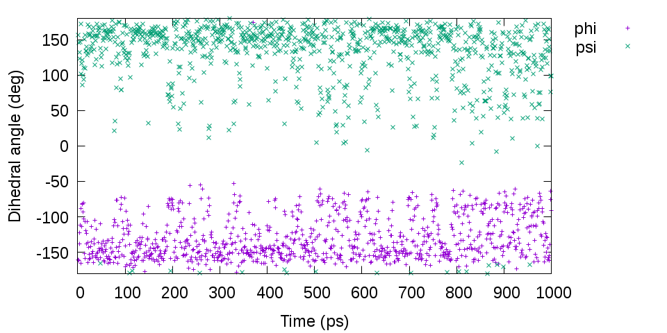
Let’s run trj_analysis. As an output file, we get output.tor, where columns 1 to 3 correspond to the snapshot index, the dihedral angle of torsion1 (φ), and torsion2 (ψ), respectively. Finally, let us plot the time courses of φ and ψ and the distribution of φ and ψ in two-dimensional space.
# Analyze the time courses of dihedral angle PHI and PSI
$ ../../bin/trj_analysis INP > log
$ ls
INP  log  output.tor

# Time courses of the dihedral angles phi and psi
$ gnuplot
gnuplot> set xlabel 'Time (ps)'
gnuplot> set ylabel 'Dihedral angle (deg)'
gnuplot> set key top outside
gnuplot> plot [][-180:180]'output.tor' u 1:2 t "phi", 'output.tor' u 1:3 t "psi"
# Distribution of the dihedral angles phi and psi
$ gnuplot
gnuplot> set xlabel 'phi (deg)'
gnuplot> set ylabel 'psi (deg)'
gnuplot> unset key
gnuplot> set size square
gnuplot> plot [-180:180][-180:180]'output.tor' u 2:3
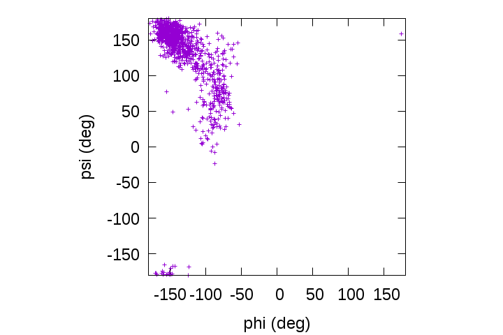
We can see that the backbone dihedral angles of the alanine-dipeptide are predominantly distributed in the β-sheet region around (φ, ψ) = (-139, 135) rather than in the α-helix region around (φ, ψ) = (-57, -47).
References
- J. Huang et al., Nat. Methods, 14, 71-73 (2017).
- J. P. Ryckaert et al., J. Comput. Phys., 23, 327-341 (1977).
- H. Andersen, J. Comp. Phys., 52, 24-34 (1983).
- G. Bussi et al., J. Chem. Phys., 126, 014101 (2007).
Written by Takaharu Mori@RIKEN Theoretical molecular science laboratory
March, 5, 2022