3.3 MD simulation of Protein G in NaCl solution
Contents
Preparation
Let’s download the tutorial file (tutorial19-3.3.zip). This tutorial consists of five steps: 1) system setup, 2) energy minimization, 3) equilibration, 4) production run, and 5) trajectory analysis. The control files for GENESIS are already included in the download file. To use the CHARMM36m force field parameters [1], we create a symbolic link to the CHARMM toppar directory (see Tutorial 2.1).
# Put the tutorial file in the Works directory
$ cd ~/GENESIS_Tutorials-2019/Works
$ mv ~/Downloads/tutorial19-3.3.zip ./
$ unzip tutorial19-3.3.zip

# Clean up the directory
$ mv tutorial19-3.3.zip TRASH

# Update the README file
$ echo "tutorial-3.3: MD simulation of Protein G in NaCl solution" >> README

# Check the contents of Tutorial 3.3
$ cd tutorial-3.3
$ ln -s ../../Data/Parameters/toppar_c36_jul21 ./toppar
$ ln -s ../../Programs/genesis-1.7.1/bin ./bin
$ ls
1_setup     3_equilibrate  5_analysis  bin
2_minimize  4_production   benchmark   toppar
One of the aims of this tutorial is to help you think about how to perform efficient calculations. To do this, we first need to know the architecture of the CPU in the computer in advance. We assume that you are using a typical Linux workstation. Let’s review the CPU information on the computer. You can use the following command (or the lscpu command) to get the CPU model, number of physical CPUs, number of cores in one physical CPU, and number of logical processors.
# Check the CPU model
$ grep 'model name' /proc/cpuinfo | uniq
model name : Intel(R) Xeon(R) CPU E5-2670 0 @ 2.60GHz

# Check the number of physical CPUs
$ grep physical.id /proc/cpuinfo | sort -u | wc -l
2

# Check the number of cores in one physical CPU
$ grep cpu.cores /proc/cpuinfo | sort -u
cpu cores : 8

# Check the number of logical processors
$ grep processor /proc/cpuinfo | wc -l
16
This example shows that the computer is equipped with an Intel Intel Xeon E5-2670 processor. There are two physical CPUs, each of which has 8 CPU cores. Thus, there are 16 CPU cores in total. This CPU architecture can be pictured as follows. Please try to draw a similar picture for your case.
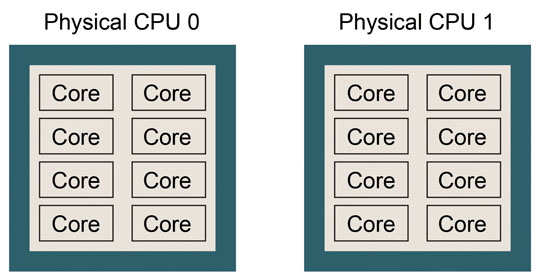
If number of logical processors is twice the (number of physical CPUs) * (number of cores in one physical CPU), hyper-threading might be turned on, which means that the number of logical processors is virtually doubled. If so, performance of GENESIS may suffer.
1. Setup
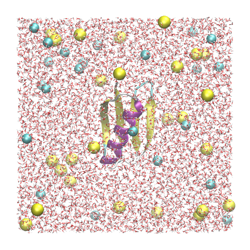
In this tutorial, we will simulate protein G using the all-atom model. The detailed setup scheme of the system has already been described in Tutorial 2.3 and will not be covered here. Since we will create symbolic links to the files and directories obtained in Tutorial 2.3, please finish that first, if you have not yet done. The protein is solvated in a 150 mM NaCl solution with a box size of 64 Å × 64 Å × 64 Å, resulting in a total number of 24,552 atoms in the system. We have ionized.pdb and ionized.psf as input files for GENESIS. Since the system is twice as large as in Tutorial 3.2, there will be much computational cost for the MD simulation.
# Change directory for the system setup
$ cd 1_setup
$ ln -s ../../tutorial-2.3/* ./
$ ls
1_oripdb  2_modpdb  3_psfgen  4_solvate  5_ionize  toppar

$ ls ./5_ionize
build.tcl  ionized.pdb  ionized.psf  log
ionized.pdb
2. Minimization
First, we perform a 2,000-step energy minimization with the steepest descent (SD) method. We use the CHARMM C36m force field parameters. The particle mesh Ewald method (PME) [2] is used to compute the long-range interactions. The scheme is the same as in Tutorial 3.2. Let’s execute spdyn for the control file INP. The following command uses 4 MPI processors and 4 OpenMP threads, that is, a total of 16 CPU cores. It will take about 1 minute to finish the calculation.
# Change directory for the energy minimization
$ cd ../2_minimize

# Run energy minimization
$ export OMP_NUM_THREADS=4
$ mpirun -np 4 ../bin/spdyn INP > log

# Check the trajectory
$ vmd ../1_setup/5_ionize/ionized.pdb -psf ../1_setup/5_ionize/ionized.psf -dcd min.dcd
3. Equilibration
The system is gradually equilibrated in three steps as in Tutorial 3.2. First, we perform a 50-ps MD simulation with positional constraints on the heavy atoms of the protein (force constant = 1.0 kcal/mol/Å2) in the NVT ensemble at T = 298.15K. The equations of motion are integrated with a time step of 2 fs with the velocity Verlet algorithm, in which the SHAKE/RATTLE [3,4] and SETTLE [5] algorithms are used for the bond constraint. The temperature is controlled with the Bussi thermostat [6]. Then, we perform a 50-ps MD simulation in the NPT ensemble at T = 298.15 K and P = 1 atm with the Bussi thermostat and the barostat [7]. Positional restraints are applied to the protein backbone heavy atoms. The other simulation conditions are the same as in the first step. Finally, we perform a 50-ps MD in the NPT ensemble at T = 298.15 K and P = 1 atm , where the equations of motion are integrated with the RESPA algorithm [8] with a time step of 2.5 fs. In the RESPA integrator, the PME calculation is performed every 2 steps and the thermostat and ballostat momenta are updated every 10 steps.
# Change directory for equilibration
$ cd ../3_equilibrate

# Step1: NVT-MD with positional restraints on protein heavy atoms
$ export OMP_NUM_THREADS=4
$ mpirun -np 4 ../bin/spdyn INP1 > log1

# Step2: NPT-MD with positional restraints on protein heavy atoms
$ mpirun -np 4 ../bin/spdyn INP2 > log2

# Step3: NPT-MD with positional restraints on protein backbone heavy atoms
$ mpirun -np 4 ../bin/spdyn INP3 > log3

# Check the trajectory
$ vmd ../1_setup/5_ionize/ionized.pdb -psf ../1_setup/5_ionize/ionized.psf -dcd eq{1..3}.dcd
4. Production
Benchmark test
Now, before we go into the production run, let’s check the benchmark performance of GENESIS. Of course, if many CPU cores are available, you can expect that the simulation will finish quickly. Benchmark test will give you detailed information in advance on how many hours or days the simulation will take to finish.
# Change directory for benchmark check
$ cd ../benchmark
$ ls
INP
In the benchmark test, we measure the simulation time by changing the number of CPU cores. Our computer has 16 CPU cores as shown above. Therefore, in the following commands, we measure the time using 1, 2, 4, 8, and 16 CPU cores with various combinations of the number of MPI processors and OpenMP threads. For example, in the case of 2MPI x 2OpenMP, 4 CPU cores are used, and in the case of 4MPI x 4OpenMP, 16 CPU cores are used. Here, thread parallel computing with OpenMP is a shared memory-based calculation, and performs well within one physical CPU. Thus, the number of OpenMP threads (OMP_NUM_THREADS) is basically set less than or equal to the number of cores within one physical CPU. Please adjust the number of CPU cores according to your computer environment. Each run is just a 1,000-steps MD (2.5 ps), which is long enough to check the performance.
$ export OMP_NUM_THREADS=1
$ mpirun -np  1 ../bin/spdyn INP >  1MPIx1OpenMP
$ mpirun -np  2 ../bin/spdyn INP >  2MPIx1OpenMP
$ mpirun -np  4 ../bin/spdyn INP >  4MPIx1OpenMP
$ mpirun -np  8 ../bin/spdyn INP >  8MPIx1OpenMP
$ mpirun -np 16 ../bin/spdyn INP > 16MPIx1OpenMP

$ export OMP_NUM_THREADS=2
$ mpirun -np  1 ../bin/spdyn INP >  1MPIx2OpenMP
$ mpirun -np  2 ../bin/spdyn INP >  2MPIx2OpenMP
$ mpirun -np  4 ../bin/spdyn INP >  4MPIx2OpenMP
$ mpirun -np  8 ../bin/spdyn INP >  8MPIx2OpenMP

$ export OMP_NUM_THREADS=4
$ mpirun -np  1 ../bin/spdyn INP >  1MPIx4OpenMP
$ mpirun -np  2 ../bin/spdyn INP >  2MPIx4OpenMP
$ mpirun -np  4 ../bin/spdyn INP >  4MPIx4OpenMP
When using 16 MPI processors, the simulation was interrupted and the following error message was displayed:
Setup_Processor_Number> Cannot define domains and cells.
Smaller or adjusted MPI processors, or shorter pairlistdist,
or larger boxsize should be used.
This message indicates that 16 MPI processors cannot be used for this calculation. SPDYN uses a method in which the system is divided into multiple domains for parallel computation (domain decomposition scheme), where the number of domains must be equal to the number of MPI processors (for details, see the “Available Programs” chapter of the User Manual). This message tells you that the system could not be divided into 16 domains. In fact, the domain size is related to the pair list distance. If a short pairlistdist is specified in the control file, it may be possible to divide the system into 16 domains. However, since switching, cutoff, and pairlist distance are recommended at 10.0, 12.0, and 13.5, respectively, these should essentially remain unchanged. Thus, in most cases, the above error message indicates that the “maximum number of available MPI processors” has been reached.
Now let’s collect the timings (timers for dynamics calculations) from all log files. Timers are in seconds. On our computer, we found that the best performance is achieved with 8 MPI processors and 2 OpenMP threads.
# Gather the timing from all log files
$ grep "dynamics      =" * | sort -g -r -k 4 > timer.out
$ tail -4 timer.out
2MPIx4OpenMP:    dynamics      =      44.213
4MPIx2OpenMP:    dynamics      =      44.069
4MPIx4OpenMP:    dynamics      =      24.393
8MPIx2OpenMP:    dynamics      =      24.318
Since we ran a 2.5 ps MD simulation for each job, the timings (s/2.5 ps) are converted to ns/day with the following command.
# Convert sec/2.5ps to ns/day
$ awk '{print $1, 24*60*60*2.5*0.001/$4}' timer.out > benckmark.out
$ tail -4 benckmark.out
2MPIx4OpenMP: 4.88544
4MPIx2OpenMP: 4.9014
4MPIx4OpenMP: 8.855
8MPIx2OpenMP: 8.88231
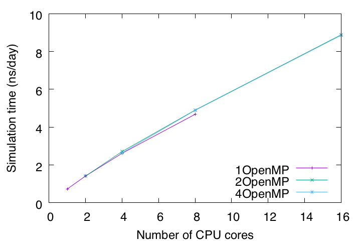
To summarize, let’s plot the timings with the number of CPU cores on the X axis and the estimated simulation time (ns/day) on the Y axis. Currently, for all-atom MD simulations with explicit solvent, 1 μs or longer is the typical length of time. According to this benchmark test, it takes about 114 days to run a 1 μs MD simulation on this computer. Such an estimate is important for making a schedule and plan to complete the simulation within a limited research period.
File size estimation
Since MD simulations generate a large amount of trajectory data, but at the same time the available disk space is finite, it is important to estimate the file size of the MD trajectory data before the production runs. In a DCD file, the coordinates of atoms are written in single-precision floating-point numbers, consuming 4 bytes x 3 = 12 bytes per atom. Now the system has 24,552 atoms. Therefore, if the MD simulation outputs 50 frames, the size of the DCD file would be approximately 15 MB (24,552 x 50 x 12 bytes). In fact, the previous step of the equilibration run generated 15 MB of data at each stage. Based on this scheme, let us estimate the file size of the trajectory data generated in the subsequent production runs.
$ du -h ../3_equilibrate/*.dcd
15M ../3_equilibrate/eq1.dcd
15M ../3_equilibrate/eq2.dcd
15M ../3_equilibrate/eq3.dcd
Production run
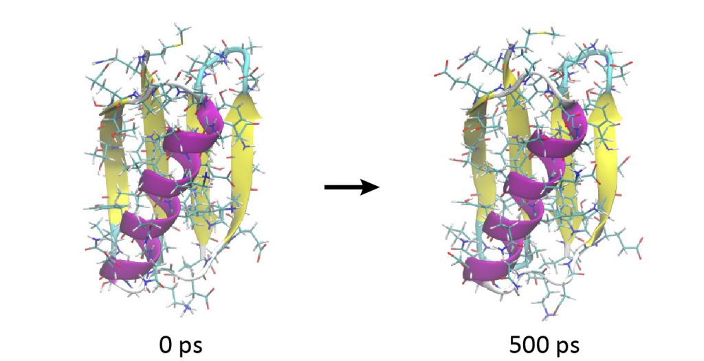
Now let’s perform the production run. The simulation conditions are the same as for the last stage of the equilibration run in Step 3, but with the position restraints turned off. Here we use 8 MPI processors and 2 OpenMP threads to achieve the best performance. We run spdyn sequentially for INP1–INP5, each corresponding to a 100-ps MD simulation. In total, we will get 500-ps MD trajectories.
# Change directory for production run
$ cd ../4_production
$ ls
INP1  INP2  INP3  INP4  INP5

# Production runs
$ export OMP_NUM_THREADS=2
$ mpirun -np 8 ../bin/spdyn INP1 > log1
$ mpirun -np 8 ../bin/spdyn INP2 > log2
$ mpirun -np 8 ../bin/spdyn INP3 > log3
$ mpirun -np 8 ../bin/spdyn INP4 > log4
$ mpirun -np 8 ../bin/spdyn INP5 > log5

# View the MD trajectories using VMD
$ vmd ../1_setup/5_ionize/ionized.pdb -psf ../1_setup/5_ionize/ionized.psf -dcd md{1..5}.dcd
Looking at the trajectory, you will observe that the protein is very stable and does not show a large conformational change during 500 ps.
5. Analysis
In this section, we will mainly learn how to process coordinates trajectory files for efficient analysis. We will also analyze the root-mean-square deviation (RMSD) of the protein using the processed DCD files.
# Change directory for analysis
$ cd ../5_analysis
$ ls
1_crd_convert_wrap  2_crd_convert_pro  3_rmsd
5.1 Make a trajectory file with PBC wrapping
When we load the coordinates trajectory data in VMD, we see that water molecules are spread out of the box and the protein is undergoing translational and rotational motions. This is a bit inconvenient for trajectory analysis. By using the “crd_convert” tool in the GENESIS program package, such trajectories can be converted to those in which all molecules are wrapped into the unit cell and the target protein is fitted to the original position.
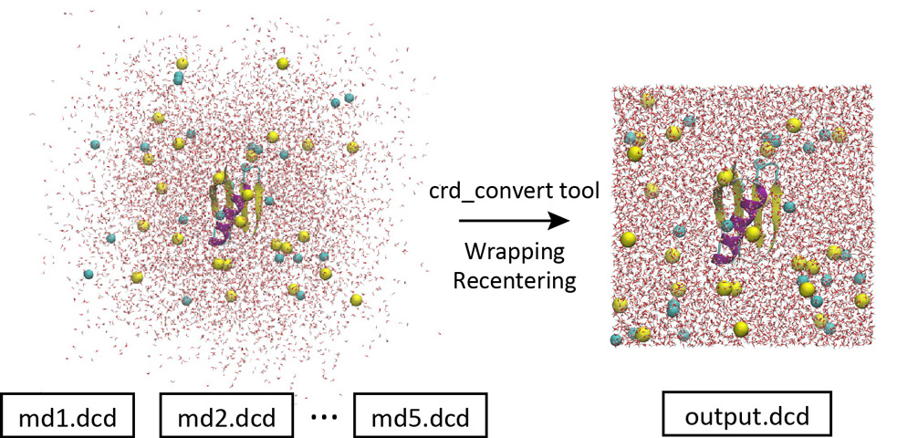
Let’s change the directory to “1_crd_convert_wrap” for this process. This directory already contains the control file. The most important part of the control file is shown below. When you convert the trajectory, the center of mass of the protein is moved to the origin (blue option) and all molecules are wrapped into the unit cell (red option). Here, psffile must be specified in the [INPUT] section for the CHARMM force field to wrap the molecules. The coordinates of all atoms in the system are output to a new DCD file “output.dcd” (green option). In the original 5 DCD files, there were a total of 1,000 snapshots (200 snapshots in each). To reduce the file size, the trajectory analysis period is set to 800 instead of the original crdout_period (purple option). Thus, the new DCD file contains a total of 250 snapshots.
[INPUT]
psffile = ../../1_setup/5_ionize/ionized.psf  # protein structure file
reffile = ../../1_setup/5_ionize/ionized.pdb  # PDB file

[OUTPUT]
pdbfile = output.pdb                          # PDB file
trjfile = output.dcd                          # trajectory file

[TRAJECTORY]
trjfile1       = ../../4_production/md1.dcd   # trajectory file
:
trjfile5       = ../../4_production/md5.dcd   # trajectory file
md_step1       = 40000                        # number of MD steps
mdout_period1  = 200                          # MD output period (crdout_period)
ana_period1    = 800                          # analysis period
repeat1        = 5

[SELECTION]
group1         = sid:PROA        # selection group 1
group2         = all             # selection group 2

[OPTION]
centering      = YES             # shift center of mass
centering_atom = 1               # atom group
center_coord   = 0.0 0.0 0.0     # target center coordinates
pbc_correct    = MOLECULE        # (NO/MOLECULE)
trjout_format  = DCD             # (PDB/DCD)
trjout_type    = COOR+BOX        # (COOR/COOR+BOX)
trjout_atom    = 2               # atom group
Let’s run crd_convert and check the resulting DCD file in VMD. This DCD file is actually useful for analyzing protein-water interactions. This is because in the original DCD file, many water molecules are spread out of the box and present in the image cells, and we do not know which water molecules are interacting with the protein. But with this new DCD, it is obvious at a glance.
# Convert the trajectory (wrap molecules)
$ ../../bin/crd_convert INP > log
$ ls
INP  log  output.pdb  output.dcd

# Check the trajectory using VMD
$ vmd output.dcd -dcd output.dcd
5.2 Make a trajectory file containing protein only
With crd_convert, it is possible to fit the Cα atoms to the initial structure, remove the water molecules, and create a new DCD file containing only protein atoms.
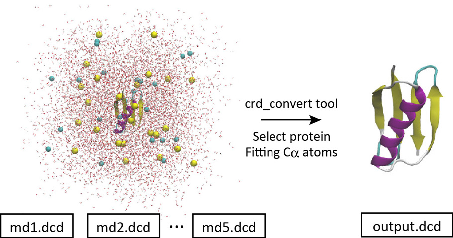
Let’s change the directory to “2_crd_convert_pro“. This directory already contains the control file. Below is the most important part of the control file. We select the protein atoms (red option) and write them to a new DCD file (output.dcd) with the Cα atoms fitted to the initial coordinates (ionized.pdb) by rigid-body translation and rotation (TR+ROT) (blue option). Since all snapshots in the original 5 DCD files were analyzed, each of which contains 200 snapshots, the resulting new DCD file contains 1,000 snapshots.
[SELECTION]
group1         = an:CA            # selection group 1
group2         = sid:PROA         # selection group 2

[FITTING]
fitting_method = TR+ROT           # NO/TR+ROT/TR/TR+ZROT/XYTR/XYTR+ZROT
fitting_atom   = 1                # atom group

[OPTION]
trjout_format  = DCD              # (PDB/DCD)
trjout_type    = COOR+BOX         # (COOR/COOR+BOX)
trjout_atom    = 2                # atom group
Let’s run crd_convert and check the resulting DCD file in VMD. This file is actually useful for analyzing the protein structure itself. This is because for such a purpose we do not need the coordinates of water molecules around the protein. In the original system, there were many water molecules. If the original DCD files were used for the trajectory analysis, it would take a very long time to just read in the coordinates of the water molecules, which would be a waste of time. In the next section, we will analyze the RMSD using the resulting DCD file instead of using the original DCD files.
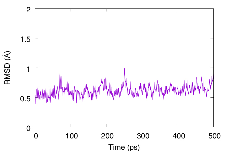
5.3 Root-mean-square deviation (RMSD)
To examine the structural stability of the protein, the rmsd_analysis tool in GENESIS is used to analyze the RMSD of the Cα atoms with respect to the initial structure. The DCD file obtained in the previous subsection is used. In the analysis, each snapshot is fitted to the initial structure (../2_crd_convert_pro/output.pdb) using rigid body translation and rotation (TR+ROT).
[INPUT]
reffile        = ../2_crd_convert_pro/output.pdb  # PDB file

[TRAJECTORY]
trjfile1       = ../2_crd_convert_pro/output.dcd  # trajectory file
md_step1       = 1000            # number of MD steps
mdout_period1  = 1               # MD output period
ana_period1    = 1               # analysis period
repeat1        = 1
:

[SELECTION]
group1         = an:CA           # selection group 1

[FITTING]
fitting_method = TR+ROT          # NO/TR+ROT/TR/TR+ZROT/XYTR/XYTR+ZROT
fitting_atom   = 1               # atom group

[OPTION]
analysis_atom  = 1               # atom group
During 500 ps, the RMSD is less than 1 Å, indicating that this protein structure is very stable. However, the RMSD is still gradually increasing and may require longer simulation runs to converge.
References
- J. Huang et al., Nat. Methods, 14, 71-73 (2017).
- T. Darden et al., J. Chem. Phys., 98, 10089-10092 (1993).
- J. P. Ryckaert et al., J. Comput. Phys., 23, 327-341 (1977).
- H. Andersen, J. Comp. Phys., 52, 24-34 (1983).
- S. Miyamoto and P. A. Kollman, J. Comput. Chem., 13, 952-962 (1992).
- G. Bussi et al., J. Chem. Phys., 126, 014101 (2007).
- G. Bussi et al., J. Chem. Phys., 130, 074101 (2009).
- M. Tuckerman et al., J. Chem. Phys., 97, 1990-2001 (1992).
Written by Takaharu Mori@RIKEN Theoretical molecular science laboratory
March 8, 2022