16.1 Cryo-EM flexible fitting for TPC2 channel
Contents
Cryo-electron microscopy (cryo-EM) is a powerful tool for determining the three-dimensional structure of biomolecules with near-atomic resolution. Flexible fitting is widely used to model atomic structures from experimentally obtained density maps [1]. One of the most commonly used methods is MD-based flexible fitting [2], which is available in ATDYN and SPDYN in the GENESIS program package [3,4]. Here we describe the basic scheme for MD-based flexible fitting using the GB/SA implicit solvent model (see also Tutorial 8.1), using cryo-EM density maps of the TPC2 channel. Fitting from a closed-form structure to an open-form density map will be demonstrated.
Preparation
Experimental data
First, let’s download the PDB file of the closed form of the TPC2 channel (PDBID: 6NQ1), and put it to the ~/GENESIS_Tutorials-2022/Data/PDB directory. We will use this structure as the initial structure of the flexible fitting. In the following example commands, we use the wget command to download the file.
# Download the PDB file of the closed form
$ cd ~/GENESIS_Tutorials-2022/Data
$ wget https://files.rcsb.org/download/6NQ1.pdb
$ mv 6NQ1.pdb ./PDB
Second, we download the experimental density map of the open form of the TPC2 channel. Let’s access to the website of EMDataResource, in which we can find experimental data deposited by cryo-EM experimentalists. The EM density map data of the open form of the TPC2 channel was determined by J. She et al (eLife, 2019), and it is registered as the “EMD-0477” in this data base. Let’s search for “0477” in the search box on the top of the page.
In the page for EMD-0477, we can see various information such as summary of the sample preparation, experimental condition, and so on. The resolution of the density map is 3.7 Å. To download the density map, click the “Download” Tab, and then “emd_0477.map.gp”. Alternatively, in the below example commands, we use the wget command for the download. Put the density map file to the ~/GENESIS_Tutorials-2022/Data/EMmap directory. We will use this density map as the target map of the flexible fitting.
# Download the EM density map file of the open form
$ wget https://ftp.wwpdb.org/pub/emdb/structures/EMD-0477/map/emd_0477.map.gz
$ gzip -d emd_0477.map.gz

$ mkdir EMmap
$ mv emd_0477.map ./EMmap
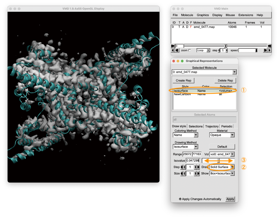
Let’s view the PDB structure and cryo-EM density map using VMD. After loading the files in VMD, we have to move the seek-bar of the “Isovalue” in the Graphical Representation window to take a look at the density map (Select [Graphics] tab in the VMD Main window > Select [Representations] > (1) Select [Isosurface] in the Graphical Representation window > (2) Select [Solid Surface] in the Draw option > (3) Move Isovalue seek-bar). We can see that the structure is already close to the density map, but not perfectly fitted to the map. In the VMD Main window, we can see that the total number of heavy atoms (Natom) in the system is about 10,000. Please keep this number in mind, which will be used later.
# Check the PDB structure and EM density map
$ vmd -ccp4 ./EMmap/emd_0477.map -pdb ./PDB/6NQ1.pdb
 Tutorial file
Let’s download the tutorial file (tutorial22-16.1.zip). In this tutorial, we use the CHARMM36m force field parameters, and we make a symbolic link to the CHARMM toppar directory (for details, see Tutorial 2.2).
# Download the tutorial file
$ cd ~/GENESIS_Tutorials-2022/Works
$ mv ~/Downloads/tutorial22-16.1.zip ./
$ unzip tutorial22-16.1.zip

# Let's clean up the directory
$ mv tutorial22-16.1.zip TRASH

# Let's take a note
$ echo "tutorial-16.1: Cryo-EM flexible fitting for TPC2 channel" >> README

# Check the contents of Tutorial 16.1
$ cd tutorial-16.1
$ ln -s ../../Data/Parameters/toppar_c36_jul21 ./toppar
$ ln -s ../../Programs/genesis-2.0.0/bin ./bin
$ ls
1_build  2_minimize  3_fitting  4_analysis  bin  toppar
1. Build the input files for GENESIS
First, input PDB and PSF files are generated using VMD (see Tutorial 2.3 or Tutorial 5.1 for details). For convenience, we also create a symbolic link to the EM density map in the same directory.
# Change directory to setup
$ cd 1_build
$ ls
build.tcl

# Make a symbolic link to the PDB and density map files
$ ln -s ../../../Data/PDB/6NQ1.pdb ./
$ ln -s ../../../Data/EMmap/emd_0477.map ./

# Generate PDB and PSF files
$ vmd -dispdev text -e build.tcl > build.log

$ ls
6NQ1.pdb   build.tcl     initial.pdb  proa.pdb
build.log  emd_0477.map  initial.psf  prob.pdb
2. Energy minimization
Before running the flexible fitting, energy minimization is carried out to remove clashes between atoms in the initial structure. The control file is already contained in the directory. Here, we simply perform the energy minimization without the EM biasing. We execute ATDYN for INP. After the calculation, min.dcd and min.rst are obtained.
# Perform energy minimization using 16 CPU cores
$ cd ../2_minimize
$ export OMP_NUM_THREADS=4
$ mpirun -np 4 ../bin/atdyn INP > log

$ ls
INP  log  min.dcd  min.rst
3. Flexible fitting
Then, we carry out the flexible fitting. The control file is already included in the directory.
# Change directory to run the simulation
$ cd ../3_fitting
$ ls
INP

# Take a look at the control file
$ less INP
The following shows the most important parts in the control file. You can understand that the flexible fitting is a kind of “restrained MD simulation”, and most parameters are common with the conventional MD simulations. We apply the EM biasing potential on the protein heavy atoms, where the force constant of the bias is set to 3Natom = 30,000 kcal/mol [5]. emfit_sigma is a resolution parameter, which is usually set to the half of the resolution of the target density map (sigma = 3.7 Å / 2 = 1.85 Å).
[INPUT]
topfile = ../toppar/top_all36_prot.rtf
parfile = ../toppar/par_all36m_prot.prm
pdbfile = ../1_build/initial.pdb
psffile = ../1_build/initial.psf
rstfile = ../2_minimize/min.rst

[SELECTION]
group1          = all and not hydrogen

[RESTRAINTS]
nfunctions      = 1
function1       = EM               # apply restraints from EM density map
constant1       = 30000            # force constant in Ebias = k*(1 - c.c.)
select_index1   = 1                # apply restraint force on protein heavy atoms

[EXPERIMENTS]
emfit           = YES                      # perform EM flexible fitting
emfit_target    = ../1_build/emd_0477.map  # target EM density map
emfit_sigma     = 1.85                     # half of the map resolution (3.7 A)
Now, let’s run ATDYN for INP. The following is an example to execute mpirun using 16 CPU cores:
# Perform flexible fitting
$ export OMP_NUM_THREADS=4
$ mpirun -np 4 ../bin/atdyn INP > log

$ ls
INP  log  run.dcd  run.pdb  run.rst
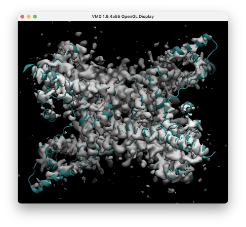
After the calculation, we obtain run.dcd, run.pdb, and run.rst, where the PDB file is the structure at the last step. The log file contains time courses of the energy and c.c. (Column 19: RESTR_CVS001). Let’s view the trajectory by using VMD. You can see that the structure is well fitted to the target density.
$ vmd -ccp4 ../1_build/emd_0477.map -pdb ../1_build/initial.pdb -psf ../1_build/initial.psf -dcd run.dcd
In this tutorial, we have done 500-steps of energy minimization and 5-ps of flexible fitting. However, in practice this should not be enough to obtain a well-fitted structure. Keep in mind that this tutorial is only a demonstration. If you try to use the same conditions as in this tutorial in your actual research, your calculations may become unstable or the fitting may not work. In such cases, please extend the minimization or simulation steps. In general, you may need more than 1,000 steps of minimization or 100 ps of flexible fitting.
4. Analysis
5.1 Cross-correlation coefficient
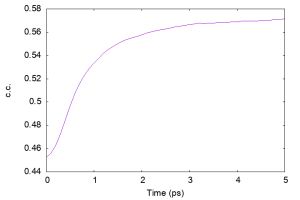
We analyze the time courses of c.c., which can be easily obtained by using the following command. We select the value in the Column 19 (RESTR_CVS001) in the log file. You can see that the c.c. is successfully increased during the fitting.
# Change directory for analysis
$ cd ../4_analysis

# Analyze time courses of c.c.
$ grep "INFO:" ../3_fitting/log | awk '{print $3, $19}' > cc.log
$ less cc.log
Let us plot the c.c. using gnuplot.
5.2 MolProbity score
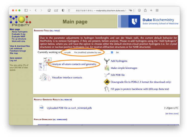
Finally, we evaluate the quality of the obtained structure. One of the commonly used criteria is the MolProbity score [6], which represents how good the structure is as a protein. It can be computed with the GUI server. Let’s access to the MolProbity Server, and upload run.pdb obtained from the flexible fitting.
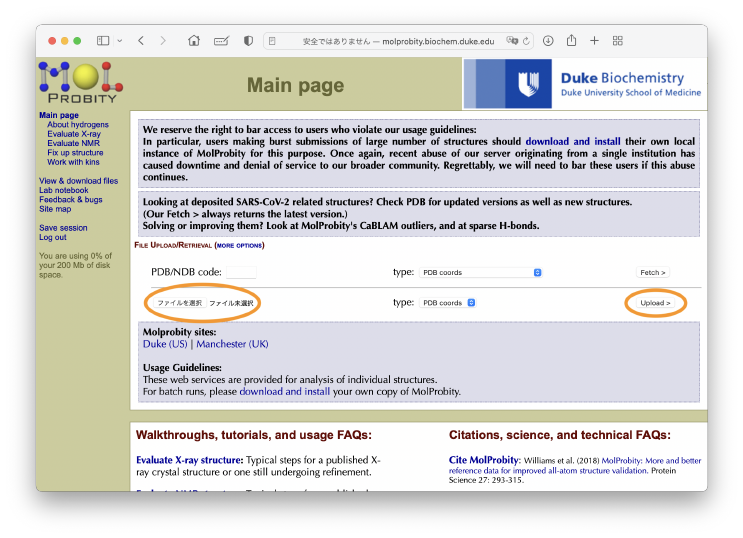 After the process, the original hydrogen atoms are removed, but the original PDB file “run.pdb” are used in the next process. We select “Currently working on [run.pdb File (modified) uploaded by user]”, and then click “analyze all-atom contacts and geometry”. In the next page, we just click the [Run programs to perform these analyses] at the bottom of the page.
 Finally, we can obtain the MolProbity score of
 run.pdb. The score 1.94 seems to be good.
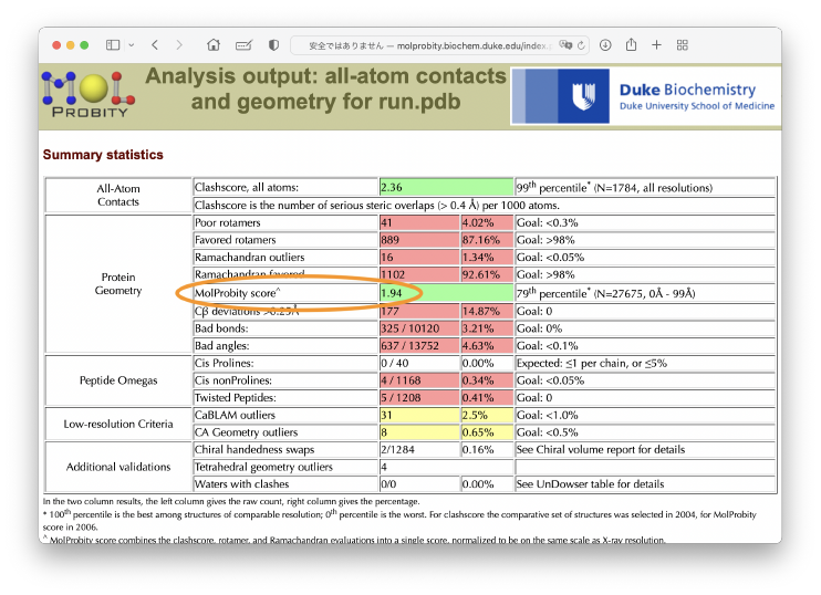
There is still a room to improve the structural quality. If we use a simulated annealing protocol in the flexible fitting, or if we further carry out an energy minimization after the flexible fitting, the score should be improved.
References
- F. Tama et al., J. Mol. Biol., 337, 985-999 (2004).
- M. Orzechowski and F. Tama, Biophys. J., 95, 5692-5705 (2008).
- O. Miyashita et al., J. Comput. Chem., 38, 1447-1461 (2017).
- T. Mori et al., Structure, 27, 161-174.e3 (2019).
- D. Matsuoka, Y. Sugita, and T. Mori (in preparation).
- V. B. Chen et al., Acta Cryst., D66, 12-21 (2010).
Written by Takaharu Mori@RIKEN Theoretical molecular science laboratory
March 26, 2022