8.1 MD simulation of Protein G in the GB/SA model
Contents
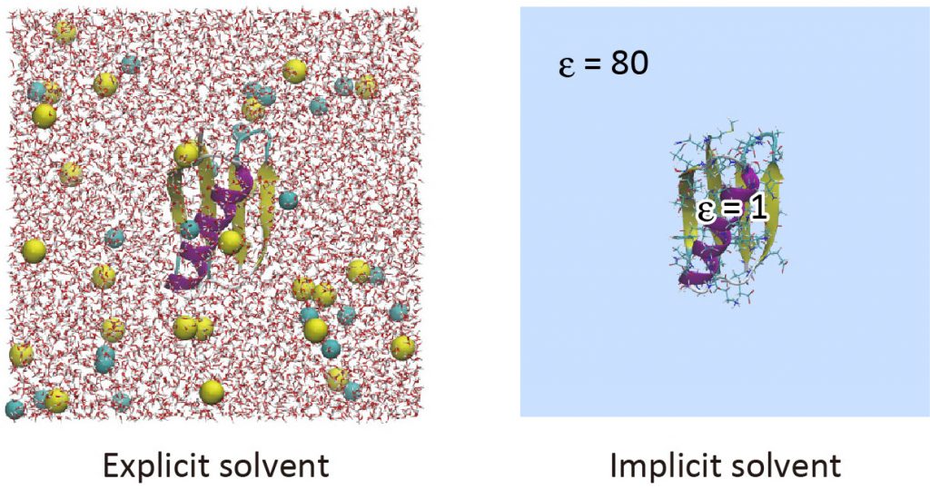
Implicit solvent models are useful to reduce computational cost in the simulation of biomolecules [1]. The GB/SA (Generalized Born/Solvent accessible surface area) model is one of the popular implicit solvent models, in which the electrostatic contribution to the solvation free energy is computed with the GB theory [2,3], and the non-polar contribution is calculated from the solvent accessible surface area [4,5]. In the GB theory, solvent molecules surrounding the solute are approximated as a continuum that has the dielectric constant of ~80. To date, various GB models have been developed such as GBSW [6], GBMV [7], HCT [8], and OBC [9]. In GENESIS, the OBC model and LCPO method [10] are used for the calculation of the GB term and SA term, respectively. The GB/SA model is introduced only in ATDYN currently, and both CHARMM and AMBER force fields are available. In this tutorial, we learn how to use the GB/SA model with the AMBER ff14SB force field parameters in GENESIS.
Preparation
First of all, download the tutorial file (tutorial22-8.1.zip). This tutorial consists of five steps: 1) system setup, 2) energy minimization, 3) equilibration, 4) production run, and 5) trajectory analysis. Control files for GENESIS are already included in the file.
# Download the tutorial file
$ cd ~/GENESIS_Tutorials-2022/Works
$ mv ~/Downloads/tutorial22-8.1.zip ./
$ unzip tutorial22-8.1.zip

# Let's clean up the directory
$ mv tutorial22-8.1.zip TRASH

# Let's take a note
$ echo "tutorial-8.1: MD simulation of Protein G in GBSA" >> README

# Check the contents of Tutorial 8.1
$ cd tutorial-8.1
$ ln -s ../../Programs/genesis-2.0.0/bin ./bin
$ ls
1_setup  2_minimize  3_equilibrate  4_production  5_analysis  bin
1. Setup
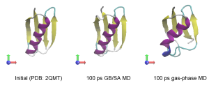
In this tutorial, we simulate Protein G in the GB/SA model. In general, GB/SA simulation is performed for a system consisting of only solute molecules (no explicit water). In the following commands, we first make a symbolic link to the PDB file of Protein G (PDB: 2QMT) in the setup directory, and then build a system by using tLEAP in the AMBER tools (see also Tutorial 5.2). Since we use the OBC2 model, we specify "set default PBradii mbondi2" in tleap.inp (see the AMBER manual). Here, we use the AMBER ff14SB force field parameters. We obtain proa.crd, proa.prmtop, and proa.pdb as the input files for GENESIS.
# Change directory for the system setup
$ cd 1_setup
$ ls
tleap.inp  vmd.tcl

# Make AMBER CRD and PRMTOP files using tLEAP
$ ln -s ../../../Data/PDB/2QMT.pdb ./
$ vmd -dispdev text -e vmd.tcl > vmd.log
$ tleap -f tleap.inp > tleap.log

$ ls
2QMT.pdb  proa.crd  proa.prmtop  tleap.log  vmd.log
leap.log  proa.pdb  tleap.inp    tmp.pdb    vmd.tcl

# View the initial structure
$ vmd -parm7 proa.prmtop -rst7 proa.crd
2. Minimization
Basically, the simulation scheme with the implicit solvent model is almost the same as those with the explicit solvent model. First, we carry out energy minimization. Let’s take a look at the control file. The following shows the most important part. In the GB/SA simulation, we usually use a longer cutoff distance than that in the explicit solvent simulation, because the electrostatic interaction is truncated at the cut-off distance. In addition, we use non-periodic boundary conditions. In this example, we use the default parameters for GBSA, where the dielectric constants of solute and solvent are set to 1.0 and 78.5, respectively, and the salt concentration is set to 0.2 mol/L, and the surface tension coefficient is 0.005 kcal/mol/Å2 (see the GENESIS user manual). Note that in GENESIS only OBC model is available currently, and the OBC2 parameters are the default setting.
# Change directory for energy minimization
$ cd ../2_minimize
$ less INP
[ENERGY]
forcefield       = AMBER   # [AMBER]
electrostatic    = CUTOFF  # [CUTOFF]
switchdist       = 23.0    # switch distance
cutoffdist       = 25.0    # cutoff distance
pairlistdist     = 28.0    # pair-list distance
implicit_solvent = GBSA    # [GBSA]

[BOUNDARY]
type             = NOBC    # [NOBC]
Then, we execute ATDYN. The following is an example command using 4 CPU cores.
# Run ATDYN
$ export OMP_NUM_THREADS=1
$ mpirun -np 4 ../bin/atdyn INP > log
3. Equilibration
In the equilibration run, we carry out a 10-ps MD simulation at 298.15K with positional restraints on the Cα atoms. The equations of motion are integrated with the velocity Verlet algorithm with the time step of 2 fs, where the SHAKE algorithm is used for bond constraint. The [ENERGY] section is same with that in the previous energy minimization. We use the Langevin thermostat to consider the random effects of the solvent on the solute atoms.
# Change directory for equilibration
$ cd ../3_equilibrate
$ less INP
[ENSEMBLE]
ensemble         = NVT       # [NVE,NVT]
tpcontrol        = LANGEVIN  # [NO,BERENDSEN,BUSSI,LANGEVIN]
temperature      = 298.15    # initial and target temperature (K)
Let’s execute ATDYN. In the log file, the solvation free energy (GB + SA terms) is shown in the 16th column.
# Run ATDYN
$ mpirun -np 4 ../bin/atdyn INP > log
4. Production run
In the production run, we carry out a 100-ps MD simulation without any restraints. The control file is almost the same as that in the previous equilibration run. The simulation time is extended, and the positional restraint is now turned off. We use INP1 for the GB/SA simulation. For comparison, we also run the gas-phase simulation using INP2, where the GB/SA term is turned off.
# Change directory for production run
$ cd ../4_production

# Run ATDYN (GBSA on)
$ mpirun -np 4 ../bin/atdyn INP1 > log1

# Run ATDYN (GBSA off)
$ mpirun -np 4 ../bin/atdyn INP2 > log2
Let’s compare the computational time between the two simulations. The computational cost of the GB/SA simulation is about six times larger than that of the gas-phase simulation. However, we can easily see that the secondary structure in Protein G is quickly broken in the gas-phase, suggesting that the solvent effect is important for the stabilization of the protein structure.
5. Analysis
Hydrogen bond formation
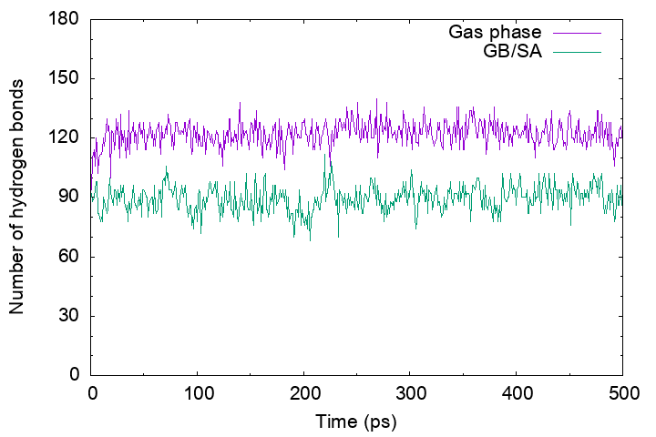
Now, we analyze the hydrogen bond formation in the GBSA and gas-phase trajectories. We use “hb_analysis” in the GENESIS analysis tool set, and the control files are already contained in the 5_analysis/H-bonds directory. In the analysis, hydrogen bond is defined if the D…A (donor…acceptor) distance is shorter than 3.4 Å, the D-H…A angle is smaller than 120°, and H-D…A angle is greater than 30°.
# Change directory for the hydrogen bond analysis
$ cd ../5_analysis
$ cd H-bonds
$ ls
INP1  INP2
[OPTION]
check_only    = NO          # only checking input files (YES/NO)
allow_backup  = NO          # backup existing output files (YES/NO)
analysis_atom = 1           # atom group for searching HB partners
target_atom   = 1           # search the HB partners from this group
hb_distance   = 3.4         # the upper limit of (D .. A) distance (default: 3.4 A)
DHA_angle     = 120.0       # the lower limit of (D-H .. A) angle (default: 120 deg.)
HDA_angle     = 30.0        # the upper limit of (H-D .. A) angle (default: 30 deg.)
boundary_type = NOBC        # (PBC / NOBC)
output_type   = count_snap  # (count_atom / count_snap)
                            # count_atom: number of H-bonds is output for each pair
                            # count_snap: number of H-bonds is output every snapshot
Let’s run hb_analysis:
# Run hb_analysis
$ ../../bin/hb_analysis INP1 > log1
$ ../../bin/hb_analysis INP2 > log2
Then, plot the “output_gbsa.out” and “output_gas.out“. You will see that the number of hydrogen bonds in the gas-phase MD trajectory is more than that in the GB/SA MD trajectory. This is because in the gas phase electrostatic interactions between polar groups have been enhanced by the absence of the shielding effect of the solvent, resulting in a broken secondary structure of the protein.
Secondary structure formation
We also analyze the secondary-structure formation tendency of each amino acid in Protein G using the DSSP algorithm. Please, install the DSSP program in your computer, if you don’t have. DSSP has been commonly used to analyze the secondary structure of proteins. However, the program can read only one PDB file. The GENESIS program package provides an interface tool (dssp_interface) to execute DSSP for the snapshot in DCD trajectory files.
Change directory to 5_analysis/DSSP. We assume that you have installed the program in /home/user/DSSP. Before analyzing the DCD files, let’s execute dssp for the initial PDB structure. In the output data, you can see the characters “H”, “E”, “S”, “T” in the 5th column, which indicates α-helix, β-sheet, bend, and turn, respectively (for details, see the DSSP manual).
# Change directory for the analysis
$ cd ../5_analysis/DSSP
$ ls
INP1  INP2  propensity

# Run DSSP for the initial structure
/home/user/DSSP/dssp ../../1_setup/proa.pdb
By using dssp_interface, we can run the DSSP program for each snapshot in the DCD file. Sample control files are included in the directory (INP1 for GBSA, and INP2 for gas-phase). In the control file, we specify a path to the DSSP program. dssp_interface generates temporary_pdb for each snapshot, and dssp analyzes temporary_pdb. This is repeated for all snapshots.
[SELECTION]
group1         = all                     # selection group 1

[OPTION]
analysis_atom  = 1                       # protein atom group
dssp_exec      = /home/user/DSSP/dssp    # dssp binary path
temporary_pdb  = temporary_gbsa.pdb      # temporary pdb for DSSP
After the calculation, we obtain dssp_gbsa.out and dssp_gas.out from INP1 and INP2, respectively. In the output files, “raw” results obtained by DSSP for all snapshots are contained.
# Run dssp_interface for INP1 and INP2
$ ../../bin/dssp_interface INP1 > log1
$ ../../bin/dssp_interface INP2 > log2

$ ls
INP1  dssp_gas.out   log1  propensity         temporary_gbsa.pdb
INP2  dssp_gbsa.out  log2  temporary_gas.pdb
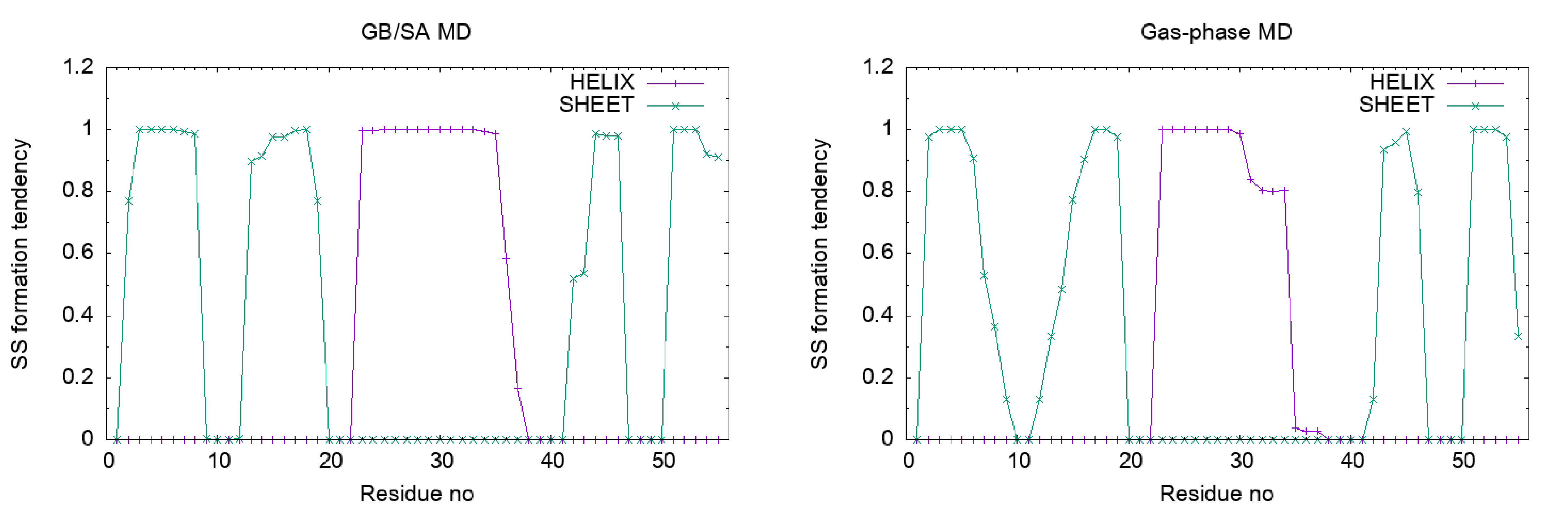
Let’s analyze the output files to calculate a secondary structure propensity of each amino acid in the protein. For this purpose, we need an additional analysis tool. The example awk program is included in the directory “propensity“. Here, calc.awk computes a rate of the secondary structure formation of each amino acid (see Appendix of this page). The α-helix and β-sheet propensities are shown in the 2nd and 3rd column of the output file, respectively. If the propensity is one, the secondary structure was formed in all snapshots.
# Change directory to analyze secondary structure propensity
$ cd propensity
$ ls
calc.awk

# Calculate the secondary structure propensity
$ awk -f calc.awk ../dssp_gbsa.out > gbsa.out
$ awk -f calc.awk ../dssp_gas.out  > gas.out
Let’s plot the results. We can see that the α-helix and β-sheet of Protein G are stable in the GB/SA simulation, while they are unstable in the gas-phase simulation.
Appendix
When you use the program calc.awk for other cases, you must take care about the following red parts. nres is the total number of amino acid residues. The characters “H” and “E” in the 5th column are counted to compute the α-helix and β-sheet propensity, respectively. Note that those characters should be in the 4th column if the PDB file does not include the chain ID.
calc.awk:
BEGIN { nres = 56; calc = 0; istr = 0; for (i=1; i<=nres; i++) freq_H[i] = 0; for (i=1; i<=nres; i++) freq_E[i] = 0 } { if ($1 == "SNAPSHOT") istr = istr + 1 if (calc == 1) { if ($5 == "H") freq_H[$1] = freq_H[$1] + 1; if ($5 == "E") freq_E[$1] = freq_E[$1] + 1 } if ($2 == "RESIDUE") calc = 1 if ($1 == nres) calc = 0 } END { printf("RESNO HELIX SHEET\n") for (i=1; i<=nres; i++) { prop_H[i] = freq_H[i]/istr; prop_E[i] = freq_E[i]/istr; printf("%5d %8.5f %8.5f\n",i, prop_H[i], prop_E[i]) } }
References
- T. Mori et al., BBA-Biomembranes, 1858, 1635-1651 (2016).
- W. C. Still et al., J. Am. Chem. Soc., 112, 6127-6129 (1990).
- D. Bashford and D. A. Case, Annu. Rev. Phys. Chem., 51, 129-152 (2000).
- D. Eisenberg and A. D. McLachlan, Nature, 319, 199-203 (1986).
- T. Ooi et al., Proc. Natl. Acad. Sci. U.S.A., 84, 3086-3090 (1987).
- W. Im et al., J. Comput. Chem., 24, 1691-1702, (2003).
- M. S. Lee et al., J. Chem. Phys., 116, 10606 (2002).
- G. D. Hawkins et al., J. Phys. Chem., 100, 19824-19839 (1996).
- A. Onufriev et al., Proteins, 55, 383-394 (2004).
- J. Weiser et al., J. Comput. Chem. 20, 217-230 (1999).
Written by Takaharu Mori@RIKEN Theoretical molecular science laboratory
March 22, 2022