GENESIS

1.3 Coarse-grained MD simulation with the Go model

Files for this turotial (tutorial-1.3.tar.gz)

Coarse-grained models are useful for investigating long-term dynamics of biomolecules with time scales (typically microseconds to seconds) difficult to access by MD simulations with atomistic models. Here, we provide a step-by-step tutorial for using a coarse-grained model with GENESIS. We simulate the folding/unfolding of protein G using a Go-model potential energy function developed by Karanicolas and Brooks (J. Karanicolas and C. L. Brooks III, 2002 ) .

The simulation input files can be found in the top of this page. Additionally, this tutorial also guides you through all the steps to produce simulation input files by yourself. This tutorial assumes that the archive file is extracted into a tutorial-1.3 folder, and each of the paragraph is done in it’s corresponding subfolder.

# make a new directory to do this tutorial
$ mkdir tutorial-1.3
$ cd tutorial-1.3

# extract the archive into the tutorial folder
$ tar xzf /path/to/tutorial-1.3.tar.gz
$ ls
1_construction 2_production 3_analysis

# verify the initial PDB structure
$ cd 1_construction
$ vmd 1pgb.pdb

1.3.1 Constructing a simulation system

The Go-model by Karanicolas and Brooks (J. Karanicolas and C. L. Brooks III, 2002 , 2003 ) is based on a minimalistic representations of a protein, where each amino acid residue is a bead located at the alpha carbon (Cα) atom position. The potential energy function is given in section 5.1 of the GENESIS manual. Although the function is almost same as that of CHARMM force field, there are several exceptions:

1. there are no electrostatic terms;
2. the vdW terms are divided into two terms for native contacts and non-native contacts, where the native contacts have 12-10-6 type attractive potential, while the non-native contacts have 12 type repulsive potential.

In this step, we generate a parfile (parameter file) and a topfile (topology file) for this Go-model using MMTSB web service. Then, using VMD we create a psffile (protein structure file) from the generated files that is required for GENESIS simulations.

To build a simulation system, we start from downloading a PDB file of protein G from the RCSB Protein Data Bank (already provided as 1_construction/1pgb.pdb). You can download the PDB file via a web browser, or directly by using the command line.

# change to the construction directory
$ cd /path/to/1_construction

# download the PDB file (PDB code 1PGB)
$ curl -o 1pgb.pdb http://files.rcsb.org/download/1PGB.pdb

The downloaded PDB file has to be “cleaned” by removing all but ATOM entries before submitting to MMTSB web service.

# "clean" the file by deleting the entries other than ATOM
$ grep -e "^ATOM" 1pgb.pdb >1pgb_edited.pdb

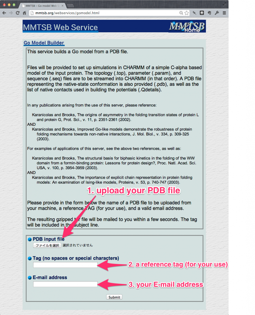
The submission to MMTSB web service consists of three stages:

1. upload the “cleaned” PDB file (1_construction/1pgb_edited.pdb);
2. give a reference tag (i.e. 1pgb);
3. enter your e-mail address.

After the submission, a tar-ball file (already provided in 1_construction/1pgb.tar) with pdbfile, parfile and topfile among others (GO_1pgb.pdb, GO_1pgb.param and GO_1pgb.top, respectively) will be emailed. Extract the tar-ball file into the working directory.

# extract the tar-ball file
$ tar xf /path/to/1pgb.tar

In this tutorial, we simulate a single-chain protein. However, if the protein of interest contains multiple chains, then the BOND, ANGLE, DIHEDRAL and NBFIX parameters including the terminal atoms between separate chains in *.param file and “Bond CA +CA” information in *.top file should be corrected manually. Later, the lack of the bond between two chains should be visually confirmed in vmd.

A VMD script (1_construction/setup.tcl) is provided to build the GO model below:

##### read pdb
mol load pdb GO_1pgb.pdb

##### replace residue names with G1, G2, G3, ...
set all [atomselect top all]
set residue_list [lsort -unique [$all get resid]]
foreach i $residue_list {
    set resname_go [format "G%d" $i]
    set res [atomselect top "resid $i" frame all]
    $res set resname $resname_go
}

$all writepdb tmp.pdb

##### generate PSF and PDB files
package require psfgen
resetpsf
topology GO_1pgb.top

segment PROT {
 first none
 last none
 pdb tmp.pdb
}
regenerate angles dihedrals
coordpdb tmp.pdb PROT

# move system origin to center of mass
$all moveby [vecinvert [measure center $all weight mass]]

# write psf and pdb files
writepsf go.psf
writepdb go.pdb

exit

The script consists of three parts:

1. the PDB file created by MMTSB web service is read and the residue names are replaced with special names for the Go-model (G1, G2, G3, …). These replacements are required to match the residue names to those defined in topfile (1_construction/GO_1pgb.param);
2. the molecule is moved so that the center of mass is at the origin;
3. psfgen plugin is called to generate psffile (1_construction/go.psf) and pdbfile (1_construction/go.pdb) .

The script can be run by VMD:

$ vmd -dispdev text <setup.tcl | tee run.out

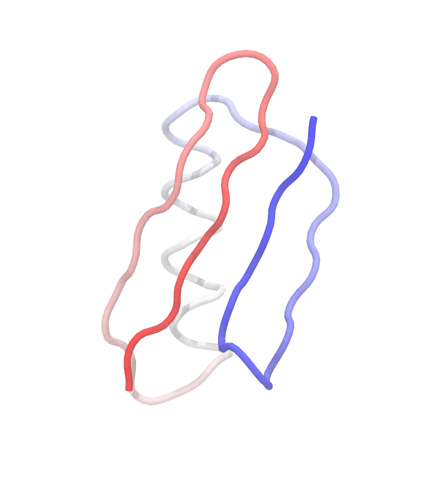
It is always a good idea to inspect the final structure visually. We can visualize the structure with VMD by specifying psffile (1_construction/go.psf) and pdbfile (1_construction/go.pdb) together:

$ vmd -psf go.psf -pdb go.pdb

If the building has successfully finished, the structure looks like this ( the coloring might differ):

1.3.2 Production simulation

Contrary to atomistic model simulations, coarse-grained simulations are not so sensitive to the initial configuration. So we perform a production simulation without minimization or equilibration.

The following command performs a 5×10⁸ step production simulation with atdyn:

# change to the production directory
$ cd /path/to/2_production/

# set the number of OpenMP threads
$ export OMP_NUM_THREADS=1

# perform production simulation with ATDYN by using 8 MPI processes
$ mpirun -np 8 atdyn run.inp | tee run.out

The control file (run.inp) contains several sections, such as [INPUT], [OUTPUT], and [ENERGY], where we can specify the control parameters for the simulation. In [INPUT] section, topfile (topology file), parfile (parameter file), psffile (protein structure file), pdbfile (the initial structure) are set (see section 4.1 of GENESIS manual for an explanation of each input file).

In the [ENERGY] section, we specify the parameters related to the energy and force evaluation. Here, KBGO is specified for the Go-model of Karanicolas and Brooks (forcefield=KBGO). This value turns on the special 12-10-6 type vdW interactions for native contacts. For the cutoff, very large values are set (switchdist=997, cutoffdist=998, pairlistdist=999) to perform a “non-cutoff” simulation.

The [DYNAMICS] section turns on the molecular dynamics engine of atdyn. For the Go-model with SHAKE constraints, time step can be 20 fs.

Note: In the case of KBGO, rigid_bond=YES tries to constrain all bonds in the molecule with SHAKE algorithm.  Generally, convergence of SHAKE becomes more difficult as molecule is bigger because the number of bonds involved in SHAKE increases. If you were simulatioting a large molecule than protein G and would likt to improve the convergence, please try a shorter timestep, for example, timestep=0.010.

In the [CONSTRAINTS] section, we enable SHAKE algorithm on all bonded pairs (rigid_bond=YES). To suppress SETTLE algorithm applied for non-existent TIP3P water molecules, we disable it explicitly (fast_water=NO). The tolerance for SHAKE is rather large compared to atomistic simulations (shake_tolerance=1.0e-6).

In the [ENSEMBLE] section, LANGEVIN thermostat is chosen for an isothermal simulation with the friction constant of 1.0 ps^-1.

Finally, in the [BOUNDARY] section, no boundary condition is imposed in this system.

[INPUT]
topfile = ../1_construction/GO_1pgb.top       # topology file
parfile = ../1_construction/GO_1pgb.param     # parameter file
psffile = ../1_construction/go.psf            # protein structure file
pdbfile = ../1_construction/go.pdb            # PDB file

[OUTPUT]
dcdfile = run.dcd                             # DCD trajectory file
rstfile = run.rst                             # restart file

[ENERGY]
forcefield      = KBGO
electrostatic   = CUTOFF
switchdist      = 997.0                       # in KBGO, this is ignored
cutoffdist      = 998.0                       # cutoff distance
pairlistdist    = 999.0                       # pair-list cutoff distance
table           = NO                          # usage of lookup table

[DYNAMICS]
integrator      = LEAP                        # [LEAP,VVER]
nsteps          = 100000000                   # number of MD steps
timestep        = 0.020                       # timestep (ps)
eneout_period   = 10000                       # energy output period
rstout_period   = 10000                       # restart output period
crdout_period   = 10000                       # coordinates output period
nbupdate_period = 10000                       # nonbond update period

[CONSTRAINTS]
rigid_bond      = YES                         # in KBGO, all bonds are constrained
fast_water      = NO                          # settle constraint
shake_tolerance = 1.0e-6                      # tolerance (Angstrom)

[ENSEMBLE]
ensemble        = NVT                         # [NVE,NVT,NPT]
tpcontrol       = LANGEVIN                    # thermostat
temperature     = 325                         # initial and target
                                              # temperature (K)
gamma_t         = 0.01                        # thermostat friction (ps-1)
                                              # in [LANGEVIN]
[BOUNDARY]
type            = NOBC                        # [PBC, NOBC]

1.3.3 Analysis: RMSD calculation

For the analysis, we use crd_convert which is one of the post-processing programs in GENESIS package. crd_convert is an utility to calculate various quantities from a trajectory. The following commands calculate RMSD of the simulation trajectory.

# change to the analysis directory
$ cd /path/to/3_analysis/

# set the number of OpenMP threads
$ export OMP_NUM_THREADS=1

# perform analysis with crd_convert
$ crd_convert run.inp | tee run.out

The control file for the RMSD calculation is shown below. In the [TRAJECTORY] section, we set the input trajectory file as trjfile1=../2_production/run.dcd.

In the [SELECTION] section, we define a group (group1) of all beads in the model which are fitted for the RMSD calculation. In the [FITTING] section, the fitting method is specified. In this case, the translations TR and rotations ROT are allowed for the fitting. Finally the RMSD output file (rmsfile=run.rms) is set in the [OUTPUT] section.

[INPUT]
psffile = ../1_construction/go.psf  # protein structure file
reffile = ../1_construction/go.pdb  # PDB file

[OUTPUT]
rmsfile = run.rms                   # RMSD file

[TRAJECTORY]
trjfile1 = ../2_production/run.dcd  # trajectory file
md_step1 = 100000000                # number of MD steps
mdout_period1 = 10000               # MD output period
ana_period1 = 1                     # analysis period
trj_format = DCD                    # (PDB/DCD)
trj_type = COOR                     # (COOR/COOR+BOX)

[SELECTION]
group1 = all                        # selection group 1

[FITTING]
fitting_method = TR+ROT             # method
fitting_atom = 1                    # atom group

[OPTION]
check_only = NO                     # (YES/NO) 

After running crd_convert, we get a RMSD file (run.rms). The first column of the file is for the time step, and the second column is for the RMSD values in Angstroms. This can be plotted with gnuplot:

$ gnuplot
gnuplot> set xlabel "Step"
gnuplot> set ylabel "RMSD [Angstrom]"
gnuplot> plot "run.rms" w lp

The noticeable fluctuations of RMSD values correspond to folding/unfolding events of the protein.

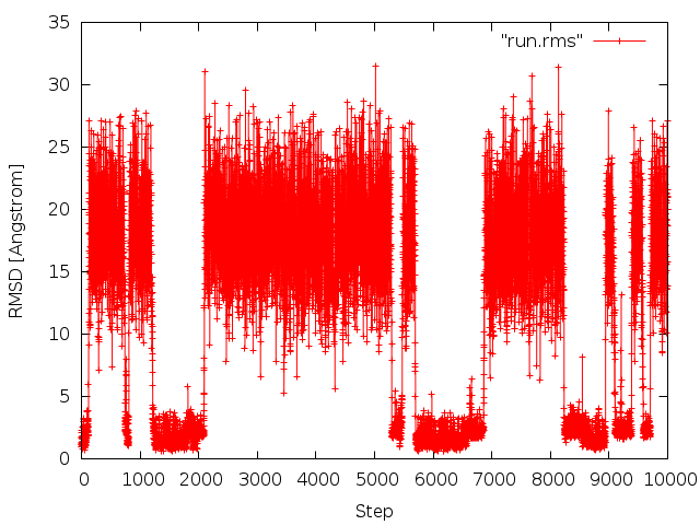
 The excact results will differ due to a different random number generator seed.

---

Written by Donatas Surblys@RIKEN Theoretical molecular science laboratory
June, XX, 2016

Updated by Yasuhiro Matsunaga@RIKEN R-CCS
May, 8, 2018

Updated by Yasuhiro Matsunaga@RIKEN R-CCS
May, 17, 2018

Updated by Yasuhiro Matsunaga@RIKEN R-CCS
May, 22, 2018