GENESIS

13.2 The closed-to-open motions of Ribose Binding Protein (RBP) with the mean-force string method

This tutorial explains using the mean-force string method [1, 2] with selected Cartesian coordinates for corrective variables (CV). Continuing with Tutorial 9.1, RBP is the target for investigating its closed-to-open motion.

0. Preparation

First of all, let’s download the tutorial file (tutorial22-13.2.zip). This tutorial consists of seven steps: 1) setup of the simulation system, 2) energy minimization, 3) equilibration, 4) longer equilibration, 5) generation of an initial pathway by targeted MD simulation, 6)replica path sampling with the mean-force string method (hereafter we call it simply “the string method”), 7) free energy calculation along the optimized pathway. Control files for GENESIS are already included in the tutorial file.

# Download the tutorial file
$ cd /home/user/GENESIS/Tutorials
$ mv ~/Downloads/tutorial22-13-2.zip ./ 
$ unzip tutorial22-13.2.zip 
$ cd tutorial-13.2
$ ls
10_rpath_equilibrate_2      1_setup                 6_target_MD
11_rpath_production         2_minimize              7_wrap_solvent
12_rpath_production_2       3_equilibrate           8_rpath_generator
13_umbrella_sampling_FC0.02 4_longer_equilibrate    9_rpath_equilibrate
14_free_energy              5_fitting               script
$ ln -sf ../../Data/Parameters/toppar_c36_jul21 ./toppar

1. Setup

2. Energy minimization

3. Equilibration

These three steps are the same as those in Tutorial 9.1 and are omitted here.

4. Longer equilibration

In actual research projects, calculations with the string method should be executed after longer equilibrations of the initial and target states.  Since this is a tutorial, only the equilibration of the initial state is shown here.

$ cd 4_longer_equilibrate
$ run.sh

5. Generation of the initial pathway by targeted MD

5.1 Preparation

As explained in Tutorial 13.1, steered/targeted MD can be executed to generate an initial pathway connecting the start (closed) and end (open) structures.  When we use selected Cartesian coordinates for CV, the targeted MD (TMD) simulation is more suitable since the method can minimize structural errors of the selected region by targeting the RMSD value. CV will be given from a TMD trajectory. Therefore, the target structure of TMD must be appropriately superimposed onto the initial structure. (The method of superimposition may vary from system to system.)

$ cd ../5_initial_pathway
$ ls
5-1_fitting 5-2_target_MD 5-3_wrap_solvent 5-4_rpath_generator

In this substep,  we will extract the final structure superimposed on the initial structure using some analysis tools implemented in GENESIS. You can perform all three processes simultaneously by running 'run.sh' in 5-1_fitting.

5.1.1. Extraction of the trajectories of equilibration.

First, we extract the last snapshot of the previous (equilibration) simulation for the closed structure using 'crd_convert'.

$ cd 5-1_fitting

The control file, 'crd_convert1.in' is as below:

[INPUT]
psffile = ../../1_setup/rbp_closed.psf
reffile = ../../1_setup/rbp_closed.pdb

[OUTPUT]
trjfile = eq4_last.pdb # The last step of the previous simulation

[TRAJECTORY]
trjfile1 = ../../4_longer_equilibrate/eq4.1.dcd
md_step1 = 4000000
mdout_period1 = 8000 
ana_period1 = 4000000
repeat1 = 1
trj_format = DCD 
trj_type = COOR+BOX
trj_natom = 0 

[SELECTION]
group1 = all

[FITTING]
fitting_method = NO # Do not apply fitting.

[OPTION]
check_only = NO
allow_backup = NO
centering = NO
centering_atom = 1
center_coord = 0.0 0.0 0.0 
pbc_correct = NO
trjout_format = PDB
trjout_type = COOR+BOX
trjout_atom = 1
split_trjpdb = NO

5.1.2. Generation of the target structure by superimposing on the initial structure.

We then superimpose the target (open) structure onto the PDB file obtained in the previous step. The control file, 'crd_convert2.in' is as below:

[INPUT]
psffile = ../../1_setup/rbp_closed.psf 
reffile = eq4_last.pdb

[OUTPUT]
trjfile = rbp_open_ref.pdb  # suporimposed target structure
rmsfile = rbp_open_ref.rms

[TRAJECTORY]
trjfile1 = ../../1_setup/rbp_open.pdb 
md_step1 = 1
mdout_period1 = 1
ana_period1 = 1
repeat1 = 1
trj_format = PDB
trj_type = COOR+BOX
trj_natom = 0

[SELECTION]
group1 = all
group2 = an:CA and (resno:108-231 or resno:269-271)

[FITTING]
fitting_method = TR+ROT
fitting_atom = 2
mass_weight = NO

[OPTION]
check_only = NO
allow_backup = NO
centering = NO
centering_atom = 1
center_coord = 0.0 0.0 0.0 
pbc_correct = NO
trjout_format = PDB
trjout_type = COOR+BOX
trjout_atom = 1 # atom group
split_trjpdb = NO # output split PDB trajectory

5.1.3. RMSD calculation between initial and target structures.

The RMSD between the initial and target structures is calculated using ‘rmsd_analysis‘.

[INPUT]
psffile = ../../1_setup/rbp_closed.psf 
reffile = eq4_last.pdb 

[OUTPUT]
rmsfile = output.rms # RMSD file

[TRAJECTORY]
trjfile1 = rbp_open_ref.pdb
md_step1 = 1 
mdout_period1 = 1 
ana_period1 = 1 
repeat1 = 1
trj_format = PDB 
trj_type = COOR+BOX
trj_natom = 0 

[SELECTION]
group1 = segid:PROA & heavy

[FITTING]
fitting_method = NO

[OPTION]
check_only = NO # only checking input files (YES/NO)
allow_backup = NO # backup existing output files (YES/NO)
analysis_atom = 1 # atom group

The RMSD can be used as the initial value of  ‘reference1 ‘ in [RESTRAINTS] of TMD at the next step. (The reference RMSD value will be updated during the TMD simulation.)

5.2. Running targeted MD

Then, we perform TMD using the superimposed target structure as 'reffile'. Since snapshots from the TMD trajectory will be selected in the next step, 'crdout_period' should be adjusted so that the number of snapshots becomes at least 10-20 times larger than the number of images for the string method.

$ cd ../5-2_target_MD
$ ls
INP run.sh

Warning: The number of steps (nsteps) in this tutorial is small because this is just a tutorial. Please enlarge the number when you execute your simulation.

[INPUT]
topfile = ../../toppar/top_all36_prot.rtf, ../../toppar/top_all36_carb.rtf
parfile = ../../toppar/par_all36m_prot.prm, ../../toppar/par_all36_carb.prm
strfile = ../../toppar/toppar_water_ions.str

psffile = ../../1_setup/rbp_closed.psf
pdbfile = ../../1_setup/rbp_closed.pdb
reffile = ../5-1_fitting/rbp_open_ref.pdb
rstfile = ../../4_longer_equilibrate/eq4.1.rst

[OUTPUT]
dcdfile = tmd.1.dcd
rstfile = tmd.1.rst

[ENERGY]
forcefield = CHARMM
electrostatic = PME
switchdist = 10.0
cutoffdist = 12.0
pairlistdist = 13.5
vdw_force_switch = YES
pme_nspline = 4
pme_max_spacing = 1.2

[DYNAMICS]
integrator = VRES 
nsteps = 400000 
timestep = 0.0025 
eneout_period = 800 
crdout_period = 800 
rstout_period = 400000 
nbupdate_period = 10 
elec_long_period = 2 
thermostat_period = 10 
barostat_period = 10 
target_md = YES 
final_rmsd = 0.5 

[CONSTRAINTS]
rigid_bond = YES

[ENSEMBLE]
ensemble = NVT
tpcontrol = BUSSI
temperature = 300.00
group_tp = YES

[BOUNDARY]
type = PBC

[SELECTION]
group1 = segid:PROA & heavy

[FITTING]
fitting_method = NO
force_no_fitting=YES
mass_weight = NO

[RESTRAINTS]
nfunctions = 1
function1 = RMSDMASS
reference1 = 6.53
constant1 = 1.0
select_index1 = 1
pressure_rmsd = yes # external force is included in virial (necessary in NPT)

5.3. Preparation for generation of an initial pathway.

In most cases,  water molecules spread out from the initial simulation box. Therefore, before executing 'rpath_generator', the trajectory should be wrapped into the box. (See section 5.1 in Tutorial 3.3)

$ cd ../5-3_wrap_solvent
$ ls
crd_convert.in run.sh

[INPUT]
psffile = ../../1_setup/rbp_closed.psf
reffile = ../../1_setup/rbp_closed.pdb

[OUTPUT]
trjfile = tmd_wrap.1.dcd

[TRAJECTORY]
trjfile1 = ../5-2_target_MD/tmd.1.dcd
md_step1 = 400000
mdout_period1 = 800 
ana_period1 = 800
repeat1 = 1
trj_format = DCD 
trj_type = COOR+BOX
trj_natom = 0 

[SELECTION]
group1 = all

[FITTING]
fitting_method = NO

[OPTION]
check_only = NO
allow_backup = NO
centering = NO
centering_atom = 1 
center_coord = 0.0 0.0 0.0
pbc_correct = MOLECULE
trjout_format = DCD
trjout_type = COOR+BOX
trjout_atom = 1 
split_trjpdb = NO

5.4. Generation of initial pathway

As explained in Tutorial 13.1, 'rpath_generator' is used to generate an initial pathway. Please add mention into the control file to apply fitting to the C-terminal domain (residue index 108-231/269-271) during the string method simulation.

$ cd ../5-4_rpath_generator
$ ls
INP run.sh

[INPUT]
dcdfile = ../5-3_wrap_solvent/tmd_wrap.1.dcd
psffile = ../../1_setup/rbp_closed.psf
pdbfile = ../5-1_fitting/rbp_open_ref.pdb
fitfile = ../5-1_fitting/rbp_open_ref.pdb

[OUTPUT]
pdbfile = {}.pdb # PDB file
rstfile = {}.rst # restart file

[SELECTION]
group1 = an:CA and segid:PROA
group2 = an:CA and (resno:108-231 or resno:269-271)

[FITTING]
fitting_method = TR+ROT
fitting_atom = 2 
mass_weight = NO 

[RPATH]
nreplica = 16
cv_atom = 1
iseed = 777
iter_reparam = 10

The CVs are stored in PDB and restart files. We can check them in each image using ‘vmd’ or other viewers.

vmd -pdb ?.pdb ??.pdb

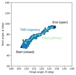
In the figure below, the images (green lines with circles) generated by rpath_generator are depicted in the collective variable space (hinge angle θ and twist angle φ). We can see that the images sparsely sampled the conformational changes occured by TMD.

6. Replica path sampling by the string method

In this step, we will perform replica path sampling starting from the initial path obtained in the previous step.

$ cd ../../6_rpath_sampling
$ ls
6-1_rpath_equilibrate 6-2_rpath_equilibrate_2 6-3_rpath_production 6-4_rpath_production_2

6.1. Equilibration of the initial pathway

Then, we perform a two-step equilibration using 16 replicas (corresponding to 16 images) to relax the all-atom structures around the images for the subsequent string method calculation.

$ cd 6-1_rpath_equilibrate
$ ls
INP run.sh

As shown in Tutorial 13.1, rpath_period=0 means that references of restraints (image coordinates) do not change during the simulation. In this stage, please do not apply the fitting to any atoms, even if the fitting is applied at 'rpath_generator' in the previous step.

The CVs are read from restart files, 'rstfile' in [INPUT] when 'use_restart=YES' is set in [RPATH] (=YES by default).

We first execute equilibration with weak force constants.

[INPUT]
topfile = ../../toppar/top_all36_prot.rtf, ../../toppar/top_all36_carb.rtf
parfile = ../../toppar/par_all36m_prot.prm, ../../toppar/par_all36_carb.prm
strfile = ../../toppar/toppar_water_ions.str
psffile = ../../1_setup/rbp_closed.psf
fitfile = ../../5_initial_pathway/5-1_fitting/rbp_open_ref.pdb
pdbfile = ../../5_initial_pathway/5-1_fitting/rbp_open_ref.pdb
reffile = ../../5_initial_pathway/5-4_rpath_generator/{}.pdb
rstfile = ../../5_initial_pathway/5-4_rpath_generator/{}.rst

[OUTPUT]
logfile = eq1.{}.log
rstfile = eq1.{}.rst
dcdfile = eq1.{}.dcd
rpathfile = eq1.{}.rpath
rpathlogfile = eq1.rpathlog

(skip)

[RPATH]
nreplica=16
rpath_period = 0
rest_function = 1
fix_terminal = YES
use_restart = YES # read CVs from restart files (default=YES)

[FITTING]
fitting_method = NO


[RESTRAINTS]
nfunctions = 1
function1 = POSI
constant1 = 0.01 0.01 0.01 0.01 0.01 \
0.01 0.01 0.01 0.01 0.01 \
0.01 0.01 0.01 0.01 0.01 \
0.01
select_index1 = 1
pressure_position = yes

6.2. Further equilibration with stronger restraints

Next, the system is equilibrated again with larger force constants, though the positional restraints would be weaker than the dihedral angle case in Tutorial 13.1. (Note: Please use enough large ‘nsteps‘ in your research project. In this tutorial,  ‘nsteps‘ is only  1,200,000 (3ns) to reduce the computational cost.)

$ cd ../6-2_rpath_equilibrate_2/
$ ls
INP run.sh

[RESTRAINTS]
nfunctions = 1
function1 = POSI
constant1 = 1.0 1.0 1.0 1.0 1.0 \
1.0 1.0 1.0 1.0 1.0 \
1.0 1.0 1.0 1.0 1.0 \
1.0 
select_index1 = 1
pressure_position = yes

In this case, CVs are Cartesian coordinates of the selected atoms.  We can convert the .rpath file of the initial pathway to PDB files by Perl scripts prepared in ../../scripts/.

$ ls ../../scripts/
rpath2pdb.pl rpath2pdb_trace.pl rpath2rms.pl
# convert the last frame of eq2.{}.rpath to pdb files. (eq2.{}.pdb)
$ ../../scripts/rpath2pdb.pl eq2

6.3. String method with fixing terminal images

After the equilibration, the pathway can be updated through the replica path sampling simulation.

$ cd ../6-3_rpath_production
$ ls
INP run.sh 

First, please set 'fix_terminal=YES' in the first several nanoseconds.

[OUTPUT]
logfile = pr1.{}.log
rstfile = pr1.{}.rst
dcdfile = pr1.{}.dcd
rpathfile = pr1.{}.rpath
rpathlogfile = pr1.rpathlog
(skip)

[RPATH]
nreplica=16
rpath_period = 1000
rest_function = 1
delta = 0.3
fix_terminal = YES

[FITTING]
fitting_method = TR+ROT
fitting_atom = 2 
mass_weight = NO 


[RESTRAINTS]
nfunctions = 1
function1 = POSI
constant1 = 1.0 1.0 1.0 1.0 1.0 \
1.0 1.0 1.0 1.0 1.0 \
1.0 1.0 1.0 1.0 1.0 \
1.0 
select_index1 = 1
pressure_position = YES

Again, the number of steps (nsteps) is small in this tutorial. Please enlarge the number when you execute the simulation in your own research. You may need to check the time course of restraint energy during the simulation.

$ grep "INFO" pr1.1.log | awk '{print $2,$16}' # printout timestep and restarint energy

pr1.{}.rpath in [OUTPUT] stores pathways of {}-th replica at each time step. You can use Perl scripts in ../../scripts/ to convert .rpath files into PDB files.

$ ls ../../scripts/
rpath2pdb.pl rpath2pdb_trace.pl rpath2rms.pl
# convert the last frame of pr1.{}.rpath to pdb files. (pr1.{}.pdb)
$ ../../scripts/rpath2pdb.pl pr1
# convert all frames of pr1.{}.rpath to pdb files with multiple models. (pr1.trace.{}.pdb)      
$ ../../scripts/rpath2pdb_trace.pl pr1

You can check the pathway using vmd or other visualization tools. This procedure is quite important. If the CVs of adjacent images are very different, it is difficult to optimize the pathway with the string method from a theoretical point of view.

$ vmd -pdb pr1.?.pdb pr1.??.pdb

You can calculate RMSDs of updated images from the initial ones using Perl script.

$ ../../scripts/rpath2rms.pl 1
what is ../../1_minim/full_open.pdb in scripts/rmsd_fit_rpath.in?

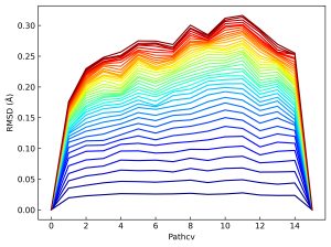
We can plot the update of the RMSD value (from blue to red) at the CV point of each image. The RMSD values of images except for two termini slightly increased during the simulation, indicating the refinement of the pathway from the initial one. 

6.4. String method with relaxing terminal images

After several nanoseconds of the replica path sampling in 6.3, the pathway will be further updated with the relaxation of the terminal images. 

$ cd ../6-4_rpath_production_2
$ ls
INP run.sh 

In this procedure, 'fix_terminal' is turned to 'NO'. Also, 'avoid_shrinkage=yes' is added to remove elements that shrink the pathway when updating terminal images.

Note: The treatment of 'avoid_shrinkage' is applied to only terminal images and will be automatically turned off when 'fix_terminal = YES'.

[RPATH]
nreplica=16
rpath_period = 1000
rest_function = 1
delta = 0.3
fix_terminal = NO
avoid_shrinkage = YES

Since this is just a tutorial, the simulation times are short. In your own simulation, please continue the calculation until the convergence of pathway updates. To check the convergence;  1) convert .rpath files (pr2.{}.rpath) to PDB files and check the change of RMSD values from the initial structure. 2) check the length of the updated pathway recorded in the .rpathlog file (pr2.rpathlog).

The final pathway should be stored for ‘mbar_analysis‘ in the next step.

grep --no-filename " 400000 " pr2.?.rpath pr2.??.rpath > pr2.last.rpath

(400000 is nsteps in this simulation, and please change this number depending on nsteps in your own simulation)

You can calculate RMSDs of updated images from the initial pathway using Perl script.

$ ../../scripts/rpath2rms.pl 2

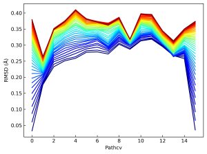
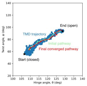
The below figure exhibits the update of the RMSD values starting from the final pathway in the previous substep. You can see the relaxation of each terminal image as an increase in the RMSD value. The other images are also refined with terminal relaxation. The initial and final pathways are plotted on the same CV-space of the figure in 5.4.

7. Free-energy calculation with the refined pathway

We already obtained the refined conformational pathway of RBP from closed to open state. In this step, we will calculate a potential mean force (PMF), a free-energy surface along with the pathway, using umbrella sampling (US) and multistate Benett-acceptance ratio (MBAR) analysis.

$ cd ../../7_free_energy 
$ ls 
7-1_umbrella_sampling 7-2_mbar_analysis 7-3_pathcv_analysis 7-4_pmf_analysis

7.1 Umbrella sampling along the pathway

7.1.1 Pathway with relaxed terminal images

Using the last snapshot of each image after the convergence of the pathway, we execute US.

$ cd 7-1_umbrella_sampling 
$ ls 
INP run.sh

The options, 'rpath_period=0' and 'fitting_method=no' should be set to the same as those in the equilibration. As shown in Tutorial 13.1, the force constants are determined so that there are sufficient overlaps in phase space, required for subsequent reweighting analysis.

[RPATH]

nreplica=16
rpath_period = 0
rest_function = 1

[FITTING]

fitting_method = no

[RESTRAINTS]

nfunctions = 1
function1 = POSI
constant1 = 0.02 0.02 0.02 0.02 0.02 \
0.02 0.02 0.02 0.02 0.02 \
0.02 0.02 0.02 0.02 0.02 \
0.02 
select_index1 = 1
pressure_position = yes

7.1.2 Pathway with fixed terminal images

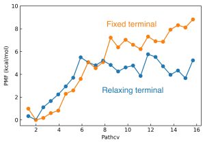
The goal of this tutorial is a comparison of free-energy landscapes for “terminal-relaxed”, and “terminal-fixed” pathways. For this purpose, we perform USs for the terminal-fixed pathway, as well as the case of the terminal-relaxed pathway in 7.1.1.

7.2 Weight calculation for each image by Multistate Benett-Acceptance Ratio (MBAR)

First, we perform MBAR analysis to calculate the weight of each image. Since we can apply these analyses to both terminal-relaxed and terminal-fixed pathways, we explain only the terminal-relaxed case. 

$ cd ../7-2_mbar_analysis
$ ls
7-2-1_crd_convert 7-2-2_mbar

7.2.1. Extraction of the trajectories of selected atoms

To perform 'mbar_analysis', only Cartesian coordinates of selected atoms are required. In addition, multiple .dcd files for each replica are not allowed as inputs. Therefore, prior to 'mbar_analysis', we generate a single trajectory file of selected atoms for each replica using 'crd_convert'. A Perl script is prepared to execute 'crd_convert' for each replica.

$ cd 7-2-1_crd_convert
$ ls 
crd_template.in run.pl
$ ./run.pl

7.2.2. Running mbar_analysis

Then we can execute ‘mbar_analysis' using the corverted trajectories.

$ cd ../7-2-2_mbar
$ ls
mbar_template.in run.pl
$ ./run.pl

In [INPUT], pathfile contains Cartesian coordinates of images and this file is generated after the convergence of the pathway.

[INPUT]
dcdfile = ../7-2-1_crd_convert/um1.{}.dcd  # a single file for each replica
pdbfile = ../../../1_setup/rbp_closed_CA.pdb
pathfile = ../../../6_rpath_sampling/6-4_rpath_production_2/pr2.last.rpath

7.3 Calculation of pathway progress using pathcv_analysis

7.3.1. Extraction of the trajectories of selected atoms with fitting

'pathcv_analysis' generates progress of the pathway from only Cartesian coordinates of selected atoms. The progress can be used for CVs of PMF. To calculate the progress value, we need to generate trajectories of selected atoms with fitting (the same way with rpath_generator).

$ cd ../../7-3_pathcv_analysis
$ ls
7-3-1_crd_convert_fit 7-3-2_pathcv_analysis

$ cd 7-3-1_crd_convert_fit
$ ls
crd_template.in run.pl

$ ./run.pl

7.3.2.Running pathcv_analysis

$ cd ../7-3-2_pathcv/
$ ls
pathcv.pr pathcv_template.in run.pl
$ ./run.pl

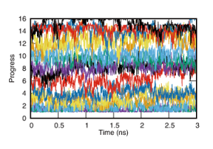
After the calculation, the progress of the pathway in each replica is generated in ‘um1.{}.pathcv’ file. We also prepare gnuplot file for checking the progress during the umbrella sampling.  An eps file, ‘pathcv.eps’ will be generated.

$ gnuplot pathcv.pr

7.4. PMF calculation using pmf_analysis

Finally, we can get PMF along with the pathway using 'pmf_analysis'. You can clearly see that the free-energy barrier, along with the close-to-open motion of RBP, is lowered by the relaxation of termini.

$ cd ../../7-4_pmf_analysis
$ ls
pmf_analysis.in
$ ${USER}/genesis-2.0/bin/pmf_analysis pmf_analysis.in > log

References

1. L. Maragliano et al., J. Chem. Phys. 125, 024106 (2006)
2. Y. Matsunaga et al., J. Phys. Chem. Lett.  7, 1446–1451 (2016)

Written by Chigusa Kobayashi@RIKEN R-CCS, Mao Oide@RIKEN CPR, and Masahiro Motohashi@RIKEN CPR

Created July 5, 2022, by CK

Updated July 27, 2022, by CK

Updated Dec 27, 2023, by MO and MM