GENESIS

13.1 The mean-force string method simulations of (Ala)₃ in water

GENESIS 1.7 or later is required for this tutorial.

Understanding conformation changes of biomolecules is a challenging problem in computational chemistry. The time scale of conventional all-atom MD simulation is usually limited to several microseconds, which is too short to observe the large conformational changes of biomolecules. The string method (also known as the replica path sampling method) is a powerful approach to study the large conformational transition between two different states of biomolecules[1-3]. The method finds the physically most probable pathway connecting two structures very efficiently, thus enabling us to examine the conformational transition of biomolecular at a feasible computational cost. In the string method, a pathway connecting the two user-defined states is represented by discrete points (called images or replicas) in the collective variables space. Then, conventional MD simulations are performed around each image to find lower free energy regions while updating images repeatedly to converge to the minimum free energy path. Currently, there are three major algorithms in the string method; (i) the string method with mean forces[1], (ii) the on-the-fly string method[2], and (iii) the string method with swarms-of-trajectories[3]. GENESIS supports (i) the string method with mean forces.

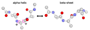
In this tutorial, we explain how to use the string method to investigate the conformational change of a small peptide (alanine tripeptide or (Ala)₃) in water. (Ala)₃ undergoes a conformational change from an alpha-helix state to a beta-sheet state. Since this process is well characterized by two dihedral angles, Φ and Ψ, we will search for the most probable pathway (called the minimum free energy path) in the subspace spanned by these two collective variables. Please note that it may take around one day or even longer to finish all simulations in this tutorial with a single-node machine. We recommend using multiple computation nodes, GPU cluster is the best choice.

All the necessary files for this tutorial can be found in the compressed zip file (tutorial22-13.1). Unpacking the file creates multiple directories inside tutorial22-13.1. We also need to make a symbolic link to the CHARMM toppar directory (see Tutorial-3.1):

# Download the tutorial file
$ cd ~/GENESIS_Tutorials-2022/Works
$ mv ~/Download/tutorial22-13.1.zip ./
$ unzip tutorial22-13.1.zip

# Let's clean up the directory
$ mv tutorial22-13.1.zip TRASH

# Let's take a note
$ echo "tutorial-13.1: The mean-force string method simulations of Ala3 in water" >> README

# Make a symbolic link to the CHARMM toppar directory
$ cd tutorial22-13.1
$ ln -s ../../Data/Parameters/toppar_c36_jul21 ./toppar
$ ln -s ../../Programs/genesis-2.0.0/bin ./
$ ls
10_pmf 2_minim_equil 4_rpath_generator 6_rpath_prod 8_mbar bin
1_setup 3_steered_md 5_rpath_equib 7_umbrella 9_pathcv_analysis toppar

Or you can copy the CHARMM toppar directory to the current tutorial directly. Please note that we provide an executable script file for every step in this tutorial (run.sh in each directory). You can finish each step just by executing the script file (“./run.sh”) in the corresponding directory.  

1. System setup

In this step, we will prepare alanine tripeptide solvated in a water box. We make PDB and PSF files of (Ala)₃ solvated in a water box (50.2 Å × 50.2 Å × 50.2 Å) by using VMD/PSFGEN (see also Tutorial-2.2 and Tutorial-3.2). Here, we skip this part and provide the final PDB and PSF files directly. 

# Change directory 
$ cd 1_setup
$ ls
end.pdb start.pdb wbox.psf

In the “1_setup” directory, we provide two PDB files: start.pdb and end.pdb, which correspond to the alpha-helix structure and beta-sheet structure of alanine tripeptide respectively. The file start.pdb, as the name suggests, is the initial structure of the simulation. While the file end.pdb represents the target states and is used as the reference file for the steered MD.

2. Energy minimization and pre-equilibration

Next, we will perform minimization and equilibration steps. The general scheme is similar to that shown in Tutorial-3.2. Here we only show the sequence of commands for performing these steps.

# Change directory
$ cd 2_minim_equil/

$ export OMP_NUM_THREADS=1

# Run minimization
$ mpirun -np 8 ../bin/spdyn INP1 > log1

# Run first NVT equilibration
$ mpirun -np 8 ../bin/spdyn INP2 > log2

# Run second NPT equilibration
$ mpirun -np 8 ../bin/spdyn INP3 > log3

3. Generating an initial pathway by steered MD

To run string simulation, firstly, we need to generate an initial pathway connecting the start (alpha-helix) and end (beta-sheet) structures. Several methods can be used to obtain this initial pathway, such as steered/targeted MD simulation, morphing, and others. Here, starting from the alpha-helix structure, we use steered MD simulation to artificially pull the structure toward the beta-sheet structure by imposing a restraint on the RMSD (Root Mean Squared Deviation) variable. A more detailed explanation of how to perform steered MD can be found in the Tutorial-9.1.

It is noted that, in the case of alanine tripeptide, the result of the steered MD simulation is very sensitive to factors such as the random seed, compiler, and hardware, therefore it is difficult to reproduce the result below (this is due to subtle fluctuations of atoms, periodicity in the dihedrals space, low free energy barriers, and so on).

The following command executes the simulation:

# Change directory
$ cd ../3_steered_md/

$ export OMP_NUM_THREADS=1

# Run steered MD
$ mpirun -np 8 ../bin/spdyn INP1 > log

The content of INP1 is shown below. Important keywords=values are indicated by red. In the steered MD simulation, reffile is required to provide the structural information of the target state. In this case, we specify reffile=../1_setup/end.pdb which represents the structure of the beta-sheet state. The steered MD scheme is turned on by steered_MD=YES. initial_rmsd is the initial RMSD value for restraint (usually RMSD value of the initial structure from the target state is specified). final_rmsd should be close to zero (exact zero might cause a crash in some cases). Fitting of the structure (to reffile) is required for RMSD calculation in order to remove the contributions from global translation and rotations. Thus, fitting_method=TR+ROT (removing TRanslation and ROTation) is specified here. Note that outputting a velocity file in steered MD is recommended since it allows GENESIS to generate better restart files.

[INPUT] 
topfile          = ../toppar/top_all36_prot.rtf
parfile          = ../toppar/par_all36m_prot.prm
strfile          = ../toppar/toppar_water_ions.str
psffile          = ../1_setup/wbox.psf
pdbfile          = ../1_setup/start.pdb
reffile          = ../1_setup/end.pdb    # structure of target state
rstfile          = ../2_minim_equil/eq2.rst

[OUTPUT] 
rstfile          = smd.rst
dcdfile          = smd.dcd
dcdvelfile       = smd.dvl  # trajectory file of velocity 
 
[ENERGY]
forcefield       = CHARMM
electrostatic    = PME
switchdist       = 10.0
cutoffdist       = 12.0
pairlistdist     = 13.5
vdw_force_switch = YES
pme_nspline      = 4
pme_max_spacing  = 1.2
 
[DYNAMICS]
integrator       = VVER
nsteps           = 600
timestep         = 0.001
eneout_period    = 2
crdout_period    = 2
velout_period    = 2
rstout_period    = 100
nbupdate_period  = 2
steered_md       = YES    # turn on steered MD
initial_rmsd     = 5.0    # initial rmsd from target structure
final_rmsd       = 0.01   # final rmsd from target structure
 
[CONSTRAINTS] 
rigid_bond       = YES
 
[ENSEMBLE] 
ensemble         = NVT
tpcontrol        = BUSSI
temperature      = 300.00
 
[BOUNDARY] 
type             = PBC
 
[SELECTION] 
group1           = rno:1-3 & heavy

[RESTRAINTS]
nfunctions       = 1
function1        = RMSD   # RMSD restraint for steered MD
reference1       = 5.0
constant1        = 100.0  # Force constant of RMSD restraint
select_index1    = 1      # Heavy atoms of (Ala)3 are used for RMSD calculation

[FITTING]
fitting_method   = TR+ROT
fitting_atom     = 1         

In the folder, we also provide a control file for the calculation of the collective variables (Φ and Ψ) with the trj_analysis tool in GENESIS. The following commands execute trj_analysis and calculate the collective variables:

# Calculate the colletive variable phi and psi from steered MD trajectory
$ ../bin/trj_analysis INP2

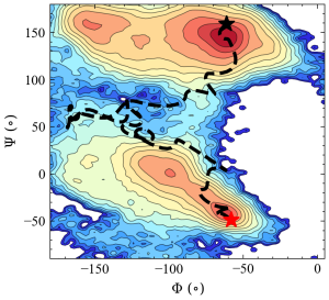
In the figure below, the trajectory of the steered MD simulation (black dash line) is projected along with the two collective variables (Φ and Ψ). The free energy surface, evaluated from very long brute-force simulations, is drawn for reference. Although the peptide successfully shifts from the initial alpha-helix structure (red star) to the final beta-sheet structure (black star), there are large fluctuations in the trajectory.

4. Preparing inputs for string simulation

In this step, we generate the necessary input files for string simulation from the steered MD trajectory. As we explained at the very beginning of this tutorial, in the string simulation, we need to represent a pathway of the conformational transition by discretized points (called images) in the collective variable space (Φ and Ψ in this tutorial). rpath_generator tool in GENESIS can prepare the images automatically by discretizing the user-provided initial pathway into a predetermined number of images. This tool works as follows: it first reads the steered MD trajectory projected onto the collective variable space. Then, trajectory snapshots are clustered, and coordinates of images are set in an equidistant manner so that the distances between adjacent images are the same. Then, the snapshot most similar (with the collective variable) to the image is extracted for each image. Finally, restart files containing the all-atom coordinates, as well as the corresponding image coordinates are written.

The following commands execute rpath_generator.

# Change directory
$ cd ../4_rpath_generator/

# Generate discreted images for string simulation
$ ../bin/rpath_generator INP > log

The content of INP is shown below. cvfile is a file containing the trajectory of steered MD projected on the collective variables (generated by trj_analysis). dcdfile and dcdvelfile are trajectory files of coordinates and velocities of the steered MD simulation, respectively. Including the trajectory file of velocities allows rpath_generator making better restart files. The number of images is specified by nreplica=16. Curly brackets {} in the [OUTPUT] section will be replaced with image indices (from 1 to 16) by GENESIS automatically. iseed is used for embedding different seeds for restart files. iter_reparam is a smoothing parameter for defining image coordinates (iter_reparam=10 is recommended).

After running the commands, 16 restart files (1.rst, …, 16.rst) and 16 PDB files(1.pdb, …, 16.pdb) are created. Restart files contain atomistic coordinates as well as coordinates of the collective variables of corresponding images. PDB files have only atomistic coordinates.

[INPUT] 
cvfile       = ../3_steered_md/smd.tor
pdbfile      = ../1_setup/start.pdb
dcdfile      = ../3_steered_md/run.dcd
dcdvelfile   = ../3_steered_md/run.dvl

[OUTPUT] 
rstfile      = {}.rst
pdbfile      = {}.pdb
 
[RPATH]  
nreplica     = 16      # number of replicas
iseed        = 31415
iter_reparam = 10

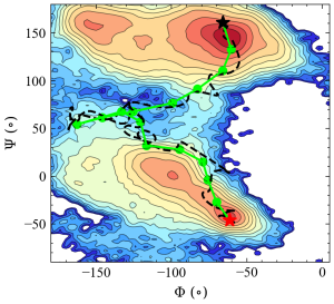
In the figure below, the images (green circles) generated by rpath_generator are depicted in the collective variable space (Φ and Ψ). It can be seen that the images are located in an equidistant manner in this 2D space.

5. Equilibration along the initial pathway

In this step, we perform a two-step equilibration using 16 replicas (corresponding to 16 images) to relax the all-atom structures around the images for the subsequent string method calculation. Weak and strong restraints on the collective variables (Φ and Ψ) are applied for each replica with reference values being specified by corresponding image coordinates successively.

# Change diretory
$ cd 5_rpath_equib/

# Run first equilibration with weak restraint
$ mpirun -np 16 ../bin/spdyn INP1 > log1

# Run second equilibration with strong restraint 
$ mpirun -np 16 ../bin/spdyn INP2 > log2

The content of INP1 is shown below. nreplica=16 in [RPATH] specifies that we perform a simulation with 16 replicas. rpath_period=0 means that references of restraints (image coordinates) do not change during the simulation. Force constants for the restraints are specified in the lists given by constants1 and constants2 (for Φ and Ψ, respectively) in [RESTRAINTS]. Each value in the list specifies the force constant of the corresponding image. In the first step, we used weak restraints (constant[12]=1.0 kcal/mol/rad²) to relax the system. Then, a strong force constant (constant[12]=100.0 kcal/mol/rad²), as recommended for string simulation, is used in the second equilibration step. Reference values for the restraints are specified by reference[12]. Here, we set these values to 0.0 because GENESIS can automatically replace these values with the coordinates of images embedded in the restart files (generated by rpath_generator). fix_teminal=YES tells GENESIS to fix the structure of the start and end state. This is useful if the terminal images correspond to crystal structures and users do not want to move them.

[INPUT] 
topfile          = ../toppar/top_all36_prot.rtf
parfile          = ../toppar/par_all36m_prot.prm
strfile          = ../toppar/toppar_water_ions.str
psffile          = ../1_setup/wbox.psf
pdbfile          = ../1_setup/start.pdb
reffile          = ../4_rpath_generator/{}.pdb 
rstfile          = ../4_rpath_generator/{}.rst

[OUTPUT] 
logfile          = eq1_{}.log
dcdfile          = eq1_{}.dcd
rstfile          = eq1_{}.rst
rpathfile        = eq1_{}.rpath

[ENERGY] 
forcefield       = CHARMM
electrostatic    = PME
switchdist       = 10.0
cutoffdist       = 12.0
pairlistdist     = 13.5
vdw_force_switch = YES
pme_nspline      = 4
pme_max_spacing  = 1.2 
contact_check    = YES 

[DYNAMICS] 
integrator       = VRES
nsteps           = 40000
timestep         = 0.0025
eneout_period    = 2000
crdout_period    = 2000
rstout_period    = 2000
nbupdate_period  = 10

[ENSEMBLE] 
ensemble         = NPT
tpcontrol        = BUSSI
temperature      = 300.0
pressure         = 1.0

[CONSTRAINTS] 
rigid_bond       = YES

[BOUNDARY] 
type             = PBC

[RPATH] 
nreplica         = 16     # number of replicas
rpath_period     = 0      # no update of the image coordinates
rest_function    = 1 2    # index of the restraint function to be used
fix_terminal     = YES    # two terminal images are always fixed

[SELECTION] 
group1           = ai:15
group2           = ai:17
group3           = ai:19
group4           = ai:25
group5           = ai:27

[RESTRAINTS]  
nfunctions       = 2

function1        = DIHED
constant1        = 1.0 1.0 1.0 1.0 1.0 1.0 1.0 1.0 \
                   1.0 1.0 1.0 1.0 1.0 1.0 1.0 1.0  
reference1       = 0.0 0.0 0.0 0.0 0.0 0.0 0.0 0.0 \
                   0.0 0.0 0.0 0.0 0.0 0.0 0.0 0.0   
select_index1    = 1 2 3 4

function2        = DIHED
constant2        = 1.0 1.0 1.0 1.0 1.0 1.0 1.0 1.0 \
                   1.0 1.0 1.0 1.0 1.0 1.0 1.0 1.0  
reference2       = 0.0 0.0 0.0 0.0 0.0 0.0 0.0 0.0 \
                   0.0 0.0 0.0 0.0 0.0 0.0 0.0 0.0  
select_index2    = 2 3 4 5

6. String simulation

Next, we perform the string simulation.

# Change diretory
$ cd ../6_rpath_prod

# Run string simulation 
$ mpirun -np 16 ../bin/spdyn INP > log

The content of INP is shown below. rpath_period in the [RPATH] specifies the duration of the time window during which the mean force is evaluated (by time-averaging). Here, the image coordinates are updated according to the estimated mean forces every rpath_period=2000 steps (corresponding to 5 ps). Typically 500-5000 steps are recommended for moderate-size biomolecules. delta in [RPATH] is the step size of the image update. A too-large delta will make the structure unstable, while a small value will result in slow convergence of the pathway. Here too, the reference values reference[12] for the restraints (the initial coordinates of images) are automatically replaced with those embedded in the restart files. The output trajectory files of the image coordinates are specified by rpathfile={}.rpath in [OUTPUT].

[INPUT] 
topfile          = ../toppar/top_all36_prot.rtf
parfile          = ../toppar/par_all36m_prot.prm
strfile          = ../toppar/toppar_water_ions.str
psffile          = ../1_setup/wbox.psf
pdbfile          = ../1_setup/start.pdb
rstfile          = ../5_rpath_equil/eq2_{}.rst
 
[OUTPUT] 
logfile          = rp_{}.log       
dcdfile          = rp_{}.dcd       
rstfile          = rp_{}.rst       
rpathfile        = rp_{}.rpath   # rpath files containing the image coordinates.

[ENERGY] 
forcefield       = CHARMM
electrostatic    = PME
switchdist       = 10.0
cutoffdist       = 12.0
pairlistdist     = 13.5
vdw_force_switch = YES
pme_nspline      = 4
pme_max_spacing  = 1.2
 
[DYNAMICS] 
integrator       = VVER
nsteps           = 2500000
timestep         = 0.002 
eneout_period    = 2000
crdout_period    = 2000
rstout_period    = 2000 
nbupdate_period  = 10
 
[CONSTRAINTS]
rigid_bond       = YES
 
[ENSEMBLE] 
ensemble         = NPT
tpcontrol        = BUSSI
temperature      = 300.0
pressure         = 1.0
 
[BOUNDARY] 
type             = PBC

[RPATH] 
nreplica         = 16       # number of replicas
rpath_period     = 2000     # period for evaluating mean-forces
delta            = 0.2      # step-size for steepest descent update of images
smooth           = 0.0      # no smoothing
rest_function    = 1 2      # index of the restraint function to be used
fix_terminal     = YES      # two terminal images are always fixed and not updated

[SELECTION] 
group1           = ai:15
group2           = ai:17
group3           = ai:19
group4           = ai:25
group5           = ai:27

[RESTRAINTS] 
nfunctions       = 2

function1        = DIHED
constant1        = 100.0 100.0 100.0 100.0 100.0 100.0 100.0 100.0 \
                   100.0 100.0 100.0 100.0 100.0 100.0 100.0 100.0
reference1       =   0.0   0.0   0.0   0.0   0.0   0.0   0.0   0.0 \
                     0.0   0.0   0.0   0.0   0.0   0.0   0.0   0.0
select_index1    = 1 2 3 4 # PHI

function2        = DIHED
constant2        = 100.0 100.0 100.0 100.0 100.0 100.0 100.0 100.0 \
                   100.0 100.0 100.0 100.0 100.0 100.0 100.0 100.0
reference2       =   0.0   0.0   0.0   0.0   0.0   0.0   0.0   0.0 \
                     0.0   0.0   0.0   0.0   0.0   0.0   0.0   0.0
select_index2    = 2 3 4 5 # PSI

The trajectories of the image coordinates, in the collective variables (Φ and Ψ) space, are written in the  "6_rpath_prod/rp_{}.rpath" files. By plotting these collective variable coordinates explicitly, we can easily track the evolution of the pathway.

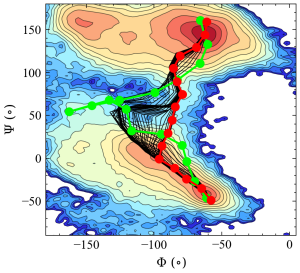
In the figure above, the green line represents the initial pathway, the black lines represent intermediate pathways during the sampling., and the red line is the final converged pathway (representing the minimum free energy path). We also provide a small shell script in the tutorial to extract the final converged pathway which is necessary for the subsequent analysis.

#!/bin/sh

# Generate the final minimum free energy pathway
if [ -f "last.path" ]; then
  rm "last.path"
fi

for ki in `seq 16`; do
  tail -n 1 rp_${ki}.rpath >> last.path
done

7. Umbrella sampling along the minimum free energy path

In the previous step, we obtained the converged pathway (minimum free energy pathway) connecting the alpha-helix and beta-sheet structures. In order to characterize the free energy profile along this pathway. we next use the umbrella sampling method to obtain the free energy surface. The umbrella sampling method has been widely used to calculate the free energy profile of the system along some collective variables. In this method, several restraint potentials are applied to the system along those collective variables, and histograms of the collective variables are obtained by using a reweighting algorithm. It should be noted that sufficient phase space overlaps are required for subsequent reweighting analysis, such as MBAR or WHAM.

# Change diretory
$ cd ../7_umbrella/

# Run umbrella sampling
$ mpirun -np 16 ../bin/spdyn INP > log

The content of INP is shown below. Again, the reference values reference[12] for the restraints (image coordinates) are automatically replaced with those embedded in the restart files (in this case, those of the last snapshots in the string simulation). Please note that rpath_period and delta in [RPATH]should be set to 0 in umbrella sampling. Also, proper force constants are required for the sufficient phase space overlap between two adjacent replicas.

[INPUT] 
topfile          = ../toppar/top_all36_prot.rtf    
parfile          = ../toppar/par_all36m_prot.prm    
strfile          = ../toppar/toppar_water_ions.str 
psffile          = ../1_setup/wbox.psf             
pdbfile          = ../1_setup/start.pdb            
rstfile          = ../6_rpath_prod/rp_{}.rst       
 
[OUTPUT] 
logfile          = umb_{}.log 
dcdfile          = umb_{}.dcd 
rstfile          = umb_{}.rst 
rpathfile        = umb_{}.rpath 

[ENERGY] 
forcefield       = CHARMM
electrostatic    = PME
switchdist       = 10.0
cutoffdist       = 12.0
pairlistdist     = 13.5
vdw_force_switch = YES
pme_nspline      = 4
pme_max_spacing  = 1.2
 
[DYNAMICS] 
integrator       = VRES
nsteps           = 2000000
timestep         = 0.0025
eneout_period    = 1000
crdout_period    = 1000
rstout_period    = 40000
nbupdate_period  = 10
 
[CONSTRAINTS] 
rigid_bond       = YES
 
[ENSEMBLE] 
ensemble         = NPT
tpcontrol        = BUSSI
temperature      = 300.0
pressure         = 1.0
 
[BOUNDARY] 
type             = PBC

[RPATH] 
nreplica         = 16 
rpath_period     = 0
delta            = 0
rest_function    = 1 2
fix_terminal     = YES

[SELECTION]
group1           = ai:15
group2           = ai:17
group3           = ai:19
group4           = ai:25
group5           = ai:27

[RESTRAINTS] 
nfunctions       = 2

function1        = DIHED
constant1        = 20.0 20.0 20.0 20.0 20.0 20.0 20.0 20.0 \
                   20.0 20.0 20.0 20.0 20.0 20.0 20.0 20.0
reference1       =  0.0  0.0  0.0  0.0  0.0  0.0  0.0  0.0 \
                    0.0  0.0  0.0  0.0  0.0  0.0  0.0  0.0
select_index1    = 1 2 3 4 # PHI

function2        = DIHED
constant2        = 20.0 20.0 20.0 20.0 20.0 20.0 20.0 20.0 \
                   20.0 20.0 20.0 20.0 20.0 20.0 20.0 20.0
reference2       =  0.0  0.0  0.0  0.0  0.0  0.0  0.0  0.0 \
                    0.0  0.0  0.0  0.0  0.0  0.0  0.0  0.0
select_index2    = 2 3 4 5 # PSI

We also provide a shell script dih.sh in the folder to calculate the collective variables (Φ and Ψ) with trj_analysis tool. By executing the script file, the collective variable file of each replica will be generated automatically.

8. MBAR analysis of the free energy profile along with the images

In the following part of this tutorial, we evaluate the free energy profile along the converged pathway by using the mbar_analysis, pathcv_analysis and pmf_analysis tools in GENESIS. First, we use mbar_analysis tool to analyze the collective variable files and calculate the relative free energy profile among the images. At the same time, we obtain the weight of each frame in every replica[5].

# Change directory
$ cd ../8_mbar/


# Calculate the relative free energy profile and unbiased weights with MBAR
$ ../bin/mbar_analysis INP > log

The content of INP is shown below. pathfile=../6_rpath_prod/last.path refers to the path file of the final converged pathway (obtained in the previous step). cvfile=../7_umbrella/umb_{}.cv refers to the collective variable files.

[INPUT] 
psffile            = ../1_setup/wbox.psf
pdbfile            = ../1_setup/start.pdb
pathfile           = ../6_rpath_prod/last.path  # file of final pathway
cvfile             = ../7_umbrella/umb_{}.cv    # collective variable file

[OUTPUT] 
fenefile           = fene.dat             # relative free energy file
weightfile         = {}.weight            # weight file

[MBAR] 
dimension          = 1       # dimension of the free energy profile
num_replicas       = 16      # number of replicas
input_type         = CV      # type of input file
nblocks            = 1
newton_iteration   = 100
temperature        = 300.0
target_temperature = 300.0
tolerance          = 10E-08
rest_function1     = 1 2
read_ref_path      = 0       # reference for each replica is defined explicitly

[RESTRAINTS] 
constant1          = 0.006092 0.006092 0.006092 0.006092 \
                     0.006092 0.006092 0.006092 0.006092 \
                     0.006092 0.006092 0.006092 0.006092 \
                     0.006092 0.006092 0.006092 0.006092
reference1         =  -58.08  -64.89  -76.07  -84.94 \
                      -96.24  -94.15  -89.72  -86.64 \
                      -84.33  -78.93  -83.10  -85.77 \
                      -80.74  -68.85  -62.55  -61.05
is_periodic1       = YES
box_size1          = 360.0

constant2          = 0.006092 0.006092 0.006092 0.006092 \
                     0.006092 0.006092 0.006092 0.006092 \
                     0.006092 0.006092 0.006092 0.006092 \
                     0.006092 0.006092 0.006092 0.006092
reference2         =  -48.95  -35.02  -24.24  -11.48 \
                       -0.95   14.45   29.34   44.57 \
                       59.94   74.49   89.46  104.77 \
                      119.45  129.44  143.63  159.10
is_periodic2       = YES
box_size2          = 360.0

$ less fene.dat
     0.0000000000000000
    -0.3488274847237864
    -0.0168096948783365
     0.1146757095587470
    -0.3476903357483172
     0.1914340993220627
     1.9528355578763374
     3.8065227433205662
     3.9759595727924788
     3.6498448820374829
     2.9165617927269176
     1.5828269715965586
     0.1552933280410853
    -1.0700710444742558
    -2.0487692029396110
    -1.3555173225438741

$ less 1.weight
     1 3.070198503406507E-005
     2 1.433995860895774E-005
     3 2.125093486984715E-005
     4 1.484653430974867E-005
     5 1.487277857447018E-005
     6 1.759031859861885E-005
     7 1.565738966114539E-005
     8 1.713826681786259E-005
     ...

# Change directory
$ cd ../9_pathcv_analysis/


# Calculate tangential and orthogonal coordinates to a pathway
$ ../bin/pathcv_analysis INP > log

[INPUT]
pathfile   = ../6_rpath_prod/last.path
cvfile     = ../7_umbrella/umb_{}.cv

[OUTPUT]
pathcvfile = {}.pathcv

[OPTION]
nreplica   = 16

$ less 1.pathcv

     1 2.0367752279467917  39.7223852590263604
     2 1.2431857784915374 -13.6652453225284543
     3 1.6107542414331801  11.0016856164995041
     4 1.1703363815449264  -7.1919998044208642
     5 1.2812352527745408 -11.6566657733450807
     6 1.5985929053871142  -7.2291767498512458
     7 1.4110629640701358 -11.8067897485528537
     8 1.8398897407868577 -17.1296149647721840

$ cd ../10_pmf

# Calculate pmf along pathcv
$ ../bin/pmf_analysis INP > log

[INPUT]
cvfile       = {}.pathcv
weightfile   = {}.weight
distfile     = {}.pathdist

[OUTPUT]
pmffile      = pathcv.pmf

[OPTION]
check_only   = NO
allow_backup = NO

nreplica     = 16
dimension    = 1
temperature  = 300
cutoff       = 200

grids1       = 0.0 17.0 30
band_width1  = 0.1
is_periodic1 = NO

After running the script, we get pathcv.pmf whose 1st column contains pathcv, which is the tangential coordinates to the final converged pathway, and 2nd column is the free energy profile. The result should like below.

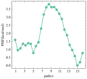
This figure shows the free energies profile along the minimum free energy path connecting the alpha-helix state (pathcv=1) and beta-sheet state (pathcv=16). Clearly, this is a two-state transition with a high free energy barrier. Please keep in mind that there might be some errors in the final free energies profiles due to the limited umbrella sampling simulation.

References

Written by Yasuhiro Matsunaga@RIKEN Computational biophysics research team
Created August 26, 2016
Updated By Weitong Ren@RIKEN Theoretical molecular science laboratory
Nov 15, 2019

Updated By Weitong Ren@RIKEN Theoretical molecular science laboratory
Mar 31, 2022