12.4 Gaussian accelerated molecular dynamics (GaMD)
Contents
The Gaussian accelerated Molecular Dynamics (GaMD) method [1,2] accelerates the conformational sampling of biomolecules by adding a harmonic boost potential to smooth the potential energy of a biological system:
\( \displaystyle U'(x) = U(x)+\Delta U^{\text{GaMD}}\left(U(x)\right),\\ \displaystyle \Delta U^{\text{GaMD}}\left(U(x)\right) = \begin{cases}\frac{1}{2}k\left\{E-U(x)\right\}^2 & (U(x) < E)\\ 0 & (U(x)\ge E),\end{cases}\)
where \(x\) is the configuration of the system, \(U\) is the potential energy, \(\Delta U^{\text{GaMD}}\) is the boost potential of GaMD, the prime represents the value biased by GaMD boosting, \(k\) is a harmonic force constant, and \(E\) is the threshold of GaMD. As shown in Figure 1, we can see that the boost potential is added to the original potential surface, which lowers the energy barrier between basins.
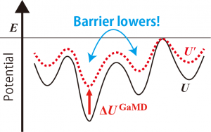
Figure 1. Scheme of GaMD boosting.
GaMD does not require predefined reaction coordinates, which is a significant advantage because expert knowledge of the biomolecular systems of interest is essential for the definition of reaction coordinates. The use of the harmonic boost potential allows us to recover the unbiased free-energy changes through cumulant expansion to the second order, which resolves the practical reweighting problems in the original accelerated MD [3]. Here, we demonstrate a GaMD simulation by employing the trialanine (Ala)3 as an example.
Note: GPU acceleration is available in GaMD simulations. If you have GPUs, we strongly recommend you to use GPUs. Please see here for GENESIS installation to GPU machines.
Preparation
First of all, let’s download the tutorial file (tutorial22-12.4). This tutorial consists of six steps: 1) system setup, 2) minimization, heating, and equilibration, 3) determination of initial parameters of GaMD by a short simulation, 4) determination of GaMD parameters with updating, 5) production run of GaMD, and 6) trajectory analysis. Control files for GENESIS are already included in the download file.
# Download the tutorial file$ cd ~/GENESIS_Tutorials-2022/Works$ mv ~/Download/tutorial22-12.4.zip ./$ unzip tutorial22-12.4.zip$ rm tutorial22-12.4.zip$ cd tutorial-12.4$ ls1_setup/ 2_equilibrate/ 3_init_parameter/ 4_update_parameter/ 5_production/ 6_analysis/
# Make a symbolic link to the CHARMM toppar directory (see Tutorial 2.2)$ ln -s ../../Data/Parameters/toppar_c36_jul21 ./toppar
# Setup the directory for binary files of GENESIS 2.0$ export GENESIS_BIN_DIR=../../../GENESIS_Tutorials-2022/Programs/genesis-2.0/bin/
In this tutorial, we use Python 3 and its libraries (NumPy, SciPy, and Matplotlib) to analyze and visualize simulation data. Please install Python 3 and the libraries to your machine.
1. Setup
In this tutorial, we perform GaMD of (Ala)3 in water. We use the same input PDB and PSF files as in Tutorial 3.2.
# Prepare the input files$ cd 1_setup$ ln -s ../../tutorial-3.2/1_setup/3_solvate/wbox.pdb ./$ ln -s ../../tutorial-3.2/1_setup/3_solvate/wbox.psf ./
2. Minimization and equilibration
We carry out energy minimization and equilibration of the system. Please refer to Tutorial 3.2, for details about input options.
# Change directory for equilibration
$ cd ../2_equilibrate
$ ls
run.sh  run1.inp  run2.inp  run3.inp  run4.inp
First, we perform a 2000-step minimization of the system to remove non-physical steric clashes. run1.inp is a control file for the minimization.
# Perform minimization
$ $GENESIS_BIN_DIR/spdyn -np 8 run1.inp > run1.out
Next, we equilibrate the system at 300 K with the constant volume during a 50-ps NVT MD simulation. Then, we carry out a 50-ps NPT MD simulation at 300 K and 1 atm using the Bussi thermostat and barostat. run2.inp and run3.inp are control files for the NVT and NPT equilibration steps, respectively.
# Perform NVT equilibration$ $GENESIS_BIN_DIR/spdyn -np 8 run2.inp > run2.out
# Perform NPT equilibration$ $GENESIS_BIN_DIR/spdyn -np 8 run3.inp > run3.out
In GaMD, the r-RESPA integrator is not available, because the long-range electrostatic potential must be calculated every time step to obtain the boosting potential. For GaMD simulations, instead of r-RESPA, we employ the velocity Verlet integrator with the long timestep. We perform a 100-ps NPT MD simulation with the 4-fs time step before GaMD simulations. For the long time step integration, the hydrogen mass repartitioning (HMR) and group temperature/pressure approach (group T/P) are required.
# Perform NPT equilibration with HMR, group T/P, and 4-fs time steps$ $GENESIS_BIN_DIR/spdyn -np 8 run4.inp > run4.out# View the trajectory using VMD$ vmd ../1_setup/wbox.psf -dcd run4.dcd
3. Determination of initial parameters of GaMD by a short simulation
In this tutorial, we use the dual boost approach of GaMD [4], in which not only the dihedral potential (including CMAP) but also the total potential of the system are independently boosted by harmonic potentials. We first determine initial parameters for GaMD dual boosting (i.e., pot_max, pot_min, pot_ave, pot_dev, dih_max, dih_min, dih_ave, dih_dev). The harmonic constant \(k\) and the threshold \(E\) in the above equation are determined from these parameters. Please refer to the GENESIS manual or the original papers of GaMD [1,2] for more detail. To obtain the initial guess of the boosting potential, we perform a short NVT MD simulation without GaMD boosting. The following command executes the simulation:
# Perform a short GaMD simulation to obtain initial parameters$ cd ../3_init_parameter $ $GENESIS_BIN_DIR/spdyn -np 8 run.inp > run.out
The following shows the most important parts in run.inp. In [GAMD] section, we set the keyword related to GaMD. GaMD is turned on by gamd = yes. boost = no means that GaMD boosts are not applied but GaMD parameters are updated from the trajectory. In this example, we use the dual boost scheme and set the threshold of GaMD to the lower bound, which are specified by boost_type = DUAL and thresh_type = LOWER, respectively. sigma0_pot and sigma0_dih are the upper limits of the standard deviation of the total potential boost and that of the dihedral potential boost, respectively. These parameters are important for accurate reweighting. The detail of the determination of these values will be explained below. We here set sigma0_pot and sigma0_dih to 6 and 1 kcal/mol, respectively. update_period in [GaMD] section is an update frequency of GaMD parameters. GaMD parameters are updated every update_period step. At the same time, the updated parameters are output to gamdfile in [OUTPUT]. For the initial determination of parameters, update_period should be set to the same as nsteps in [DYNAMICS]. Hereafter, we use the 4-fs time step integration for all GaMD simulations.
[OUTPUT]
dcdfile  = run.dcd
rstfile  = run.rst
gamdfile = run.gamd

[GAMD]
gamd          = yes
boost         = no
boost_type    = DUAL
thresh_type   = LOWER
sigma0_pot    = 6.0
sigma0_dih    = 1.0
update_period = 250000
The example of GaMD output file (gamdfile) is shown below.
STEP POT_MAX POT_MIN POT_AVE POT_DEV POT_TH POT_KC POT_KC0 DIH_MAX DIH_MIN DIH_AVE DIH_DEV DIH_TH DIH_KC DIH_KC0--------------- --------------- --------------- --------------- ---------------250000 -38059.4180 -38756.9062 -38400.5312 80.5391 -38059.4180 0.0002 0.1523 19.3442 -3.0486 6.7752 2.2532 19.3442 0.0353 0.7907
4. Determination of GaMD parameters with updating
In this step, we determine GaMD parameters by updating them at each update_period period while the boosting potentials are applied to the system. The following command executes the GaMD simulation with NVT ensemble:
# Perform a GaMD simulation to determine GaMD parameters$ cd ../4_update_parameter $ $GENESIS_BIN_DIR/spdyn -np 8 run.inp > run.out
The most important parts in run.inp are shown below. To turn on GaMD boosting, we set boost = yes in this step. The values of pot_max, pot_min, pot_ave, pot_dev, dih_max, dih_min, dih_ave, and dih_dev are initially set to the parameters determined in the previous step (i.e., the values in the last line in gamdfile). Please set the values detemined in the previous step to these parameters. We here specify the update frequency of GaMD parameters by update_period = 250. From the energy trajectory of 500 steps, the maximum, minimum, average, and standard deviation of the energy are calculated, and then the corresponding GaMD parameters are updated. The updated parameters are output to gamdfile in [OUTPUT] every update_period = 500 period.
[OUTPUT]
dcdfile  = run.dcd
rstfile  = run.rst
gamdfile = run.gamd

[GAMD]
gamd          = yes
boost         = yes
boost_type    = DUAL
thresh_type   = LOWER
sigma0_pot    = 6.0
sigma0_dih    = 1.0
update_period = 250
pot_max       = -38059.4180
pot_min       = -38756.9062
pot_ave       = -38400.5312
pot_dev       = 80.5391
dih_max       = 19.3442
dih_min       = -3.0486
dih_ave       = 6.7752
dih_dev       = 2.2532
The example of GaMD output file is shown below. Parameter updating should be continued until the parameters converge. The parameters in the last line of gamdfile are used for the production run.
STEP POT_MAX POT_MIN POT_AVE POT_DEV POT_TH POT_KC POT_KC0 DIH_MAX DIH_MIN DIH_AVE DIH_DEV DIH_TH DIH_KC DIH_KC0--------------- --------------- --------------- --------------- ---------------250 -38059.4180 -38756.9062 -38239.5312 38.4712 -38059.4180 0.0009 0.6040 19.3442 -3.0486 8.2686 2.0451 19.3442 0.0441 0.9886500 -38055.2578 -38756.9062 -38178.4102 69.8897 -38055.2578 0.0007 0.4891 19.3442 -3.0486 9.2682 2.4522 19.3442 0.0405 0.9063.........499750 -37468.2812 -38756.9062 -37715.1523 80.5094 -37468.2812 0.0003 0.3890 23.1753 -3.0486 11.8916 2.3505 23.1753 0.0377 0.9888500000 -37468.2812 -38756.9062 -37715.0977 80.5305 -37468.2812 0.0003 0.3890 23.1753 -3.0486 11.8922 2.3506 23.1753 0.0377 0.9887
5. How to determine sigma0_pot and sigma0_dih
sigma0_pot and sigma0_dih should be determined by following Miao’s protocol [1] for the highest acceleration and accurate reweighting. First, perform a short GaMD simulation with low values of sigma0_pot and sigma0_dih (e.g., both are 1.0 kcal/mol). In gamdfile, POT_KC0 (= \(k_{0P}\)) might be lower than 1.0, which means that there is room to increase boost. Increase POT_KC0 to 1.0 by adjusting sigma0_pot from 1.0 to 6.0. For the (Ala)3 system, POT_KC0 is lower than 1.0 even though sigma0_pot is set to the upper limit, 6.0 kcal/mol. For accurate reweighing, do not exceed the upper limit.
Next, perform a short GaMD simulation with the determined value of sigma0_pot. DIH_KC0 (= \(k_{0D}\)) might be lower than 1.0. Increase DIH_KC0 to 1.0 by adjusting sigma0_dih from 1.0 to 6.0. For the (Ala)3 system, DIH_KC0 becomes approximately 1.0 when sigma0_dih = 1.0. In this tutorial, sigma0_pot=6.0 and sigma0_dih=1.0 are employed.
6. Production run of GaMD
In this step, we perform 10 independent production runs of GaMD. Let’s move to the directory for production.
$ cd ../5_production $ lsmake_inp.sh
make_inp.sh is the script for generating the control files for GaMD simulations. Execute make_inp.sh.
$ bash ./make_inp.shThe script generates 10 files (run1.inp to run10.inp) with the different random seeds. The most important parts in the generated control file are shown below. Please set the parameters obtained in the previous step to pot_max, pot_min, pot_ave, pot_dev, dih_max, dih_min, dih_ave, and dih_dev. Since GaMD parameters should not be changed in production MDs, we specify update_period = 0. We notice that the frequency of output should be high, i.e., eneout_period = 25 and crdout_period = 25 in order to reweight the GaMD trajectory accurately.
[OUTPUT]
dcdfile  = run.dcd
rstfile  = run.rst
gamdfile = run.gamd

[GAMD]
gamd          = yes
boost         = yes
boost_type    = DUAL
thresh_type   = LOWER
sigma0_pot    = 6.0
sigma0_dih    = 1.0
update_period = 0
pot_max       = -37468.2812
pot_min       = -38756.9062
pot_ave       = -37715.0977
pot_dev       = 80.5305
dih_max       = 23.1753
dih_min       = -3.0486
dih_ave       = 11.8922
dih_dev       = 2.3506
Perform 10-ns GaMD simulations. If you have PC clusters or supercomputer systems, you can perform individual runs in parallel on different compute nodes, because each run is independent.
# Perform 10 GaMD simulations$ $GENESIS_BIN_DIR/spdyn -np 8 run1.inp > run1.out$ $GENESIS_BIN_DIR/spdyn -np 8 run2.inp > run2.out...$ $GENESIS_BIN_DIR/spdyn -np 8 run9.inp > run9.out$ $GENESIS_BIN_DIR/spdyn -np 8 run10.inp > run10.out
7. Analysis
7.1 Calculation of end-to-end distance
To obtain the free-energy landscape of the end-to-end distance of (Ala)3, we extract the distance from the trajectory. Let’s move to the directory for analysis.
$ cd ../6_analysis/1_calc_dist$ lsrun.sh
run.sh calculates the distance between the OY atom of residue 1 and the HNT atom of residue 3 from the GaMD trajectories (run1.dcd to run10.dcd). The values of the end-to-end distances are outputted to cv1.dat – cv10.dat.
#!/bin/bash
for i in {1..10}; dorm cv${i}.datcat << EOF > INP[INPUT]psffile = ../../1_setup/wbox.psfreffile = ../../1_setup/wbox.pdb[OUTPUT]disfile = cv${i}.dat[TRAJECTORY]trjfile1 = ../../5_production/run${i}.dcdmd_step1 = 2500000 # number of MD stepsmdout_period1 = 25 # MD output periodana_period1 = 25 # analysis periodrepeat1 = 1trj_format = DCD # (PDB/DCD)trj_type = COOR+BOX # (COOR/COOR+BOX)[OPTION]check_only = NOdistance1 = PROA:1:ALA:OY PROA:3:ALA:HNTEOFtrj_analysis ./INP > log${i}rm ./INPdone
Execute run.sh to obtain trajectories of end-to-end distance.
$ bash ./run.sh
7.2 Reweighting of the free-energy landscape of the end-to-end distance
The distribution of the end-to-end distance obtained in the previous step is not yet reweighted, that is, the free energy landscape is still imposed by the GaMD boost potentials. The unbiased probability distribution of the CV of interest can be obtained by the following equations:
\( \displaystyle p(\xi) = \frac{\int \delta (\xi-\xi(x))\exp [-\beta U(x)] dx}{\int \exp [-\beta U(x)] dx} \\ \displaystyle =\frac{\int \delta (\xi-\xi(x))\exp [\beta \Delta U^{\text{GaMD}}(x)] \exp [-\beta U'(x)] dx}{\int \delta (\xi-\xi(x)) \exp [-\beta U'(x)] dx} \frac{\int \delta (\xi-\xi(x))\exp [-\beta U'(x)] dx}{\int \exp [-\beta U'(x)] dx} \\ \displaystyle \frac{\int \exp [-\beta U'(x)] dx}{\int \exp [\beta \Delta U^{\text{GaMD}}(x)] \exp [-\beta U'(x)] dx} \\ \displaystyle = \left<\exp[\beta \Delta U^{\text{GaMD}}]\right>’_{\xi} \frac{p'(\xi)}{\left<\exp[\beta \Delta U^{\text{GaMD}}]\right>’},\)
where \(\xi\) is the CV. However, the convergence of \( \left<\exp[\beta \Delta U^{\text{GaMD}}]\right>’_{\xi} \) is very slow, which causes a large statistical error. To reduce the statistical error, the cumulant expansion to the second order has been employed for GaMD simulations [3].
We here reweight the free-energy landscape of the end-to-end distance. Let’s move to the directory for reweighting.
$ cd ../2_reweight_dist$ lscalc_pmf_1d.py plot.sh run.sh
First, we merge CV trajectories into one file.
## Get CV trajectories$ cp /dev/null cv.dat$ for i in {1..10}; do$ cat ../1_calc_dist/cv${i}.dat >> cv.dat$ done
Next, we extract the GaMD boost potentials \(\Delta U^{\text{GaMD}}\) from the GENESIS log file.
## Get boost potentials from a GENESIS log file
$ cp /dev/null out.dat
$ for i in {1..10}; do
$    grep "^INFO" ../../5_production/run${i}.out >> out.dat
$ done
The example of out.dat is shown below. The values in the 18th and 19th columns correspond to the boost potentials of the total potential and dihedral energies, respectively.
INFO: STEP TIME TOTAL_ENE POTENTIAL_ENE KINETIC_ENE RMSG BOND ANGLE UREY-BRADLEY DIHEDRAL IMPROPER CMAP VDWAALS ELECT TEMPERATURE VOLUME POTENTIAL_GAMD DIHEDRAL_GAMDINFO: 25 0.1000 -30517.1473 -37592.8055 7069.3549 12.8205 6.9719 20.2106 1.6648 9.7176 1.3316 -0.3567 4018.4266 -41650.7717 302.9330 117804.3750 2.7055 3.5978INFO: 50 0.2000 -30519.4036 -37654.5874 7126.2367 12.5775 6.6194 20.4862 1.6479 11.2502 2.1430 -0.9214 3995.9417 -41691.7543 310.1379 117804.3750 5.8359 3.1113 … … …
From out.dat and cv.dat, we can obtain the reweighted free-energy landscape by the following commands.
$ python ./calc_pmf_1d.py -t 300.0 -c 10.0 -n 1000000 --Xmin 0.0 --Xmax 14.0 --Xdel 0.5 --cv_file cv.dat --out_file out.dat --anharmcalc_pmf_1d.py reweights the free-energy landscape using the cumulant expansion and outputs the unbiased free energies in each bin, “pmf_1d.dat“. The absolute temperature, the number of samples, the minimum value of the CV, the maximum value of the CV, and the grid size of the bin for the CV are assigned by arguments of the script, “-t“, “-n“, “--Xmin“, “--Xmax“, “--Xdel“, respectively. “-c” represents the cutoff of the number of samples in each bin. If the number of samples in a certain bin is below 10, the probability (or free energy) in the bin is omitted. cv.dat and out.dat are assigned by “--cv_file” and “--out_file“, respectively. If “--anharm” argument is used, the anharmonicity of each bin is also calculated (anharm_1d.dat), which represents how the distribution in each deviates from the Gaussian distributions. The reweighting is accurate when the anharmonicity is small. The example of “pmf_1d.dat” is shown below. If the bin has no sample, its free energy is set to a large value (>10000000).
0.250000 10000019.4752750.750000 10000019.4752751.250000 10000019.4752751.750000 2.5535522.250000 1.8711532.750000 1.755753...12.250000 2.30220012.750000 4.66221913.250000 10000019.47527513.750000 10000019.475275
The reweighted free-energy landscape is shown in Figure 2. We can see that the free-energy barriers in the unreweighted PMF (i.e., biased PMF) becomes lower than those in the reweighted PMF.
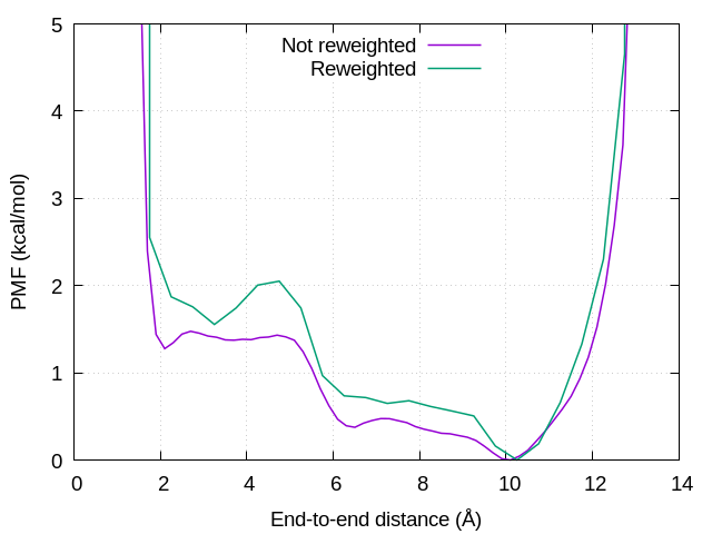
Figure 2. Free-energy landscapes of the end-to-end distance of (Ala)3. Puple and green lines represent unreweighted and reweighted free energies, respectively.
7.3 Calculation of dihedral angles
To obtain the free-energy landscape in a 2-dimensional dihedral-angle space, we calculate dihedral angles around residue 2 in (Ala)3 (Figure 3).
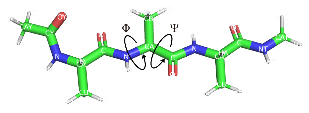
Figure 3. Dihedral angles of residue 2 in (Ala)3.
Let’s move to the directory for analysis.
$ cd ../3_calc_dihe$ lsrun.sh
run.sh calculates Φ (torsion 1) and Ψ (torsion 2) dihedral angles from the GaMD trajectories. (run1.dcd to run10.dcd). The values of the dihedrals are outputted to cv1.dat to cv10.dat.
#!/bin/bash for i in {1..10}; dorm cv${i}.datcat << EOF > INP[INPUT]psffile = ../../1_setup/wbox.psfreffile = ../../1_setup/wbox.pdb[OUTPUT]torfile = cv${i}.dat[TRAJECTORY]trjfile1 = ../../5_production/run${i}.dcdmd_step1 = 2500000 # number of MD stepsmdout_period1 = 25 # MD output periodana_period1 = 25 # analysis periodrepeat1 = 1trj_format = DCD # (PDB/DCD)trj_type = COOR+BOX # (COOR/COOR+BOX)[OPTION]check_only = NOtorsion1 = 1:ALA:C 2:ALA:N 2:ALA:CA 2:ALA:C # PHI angletorsion2 = 2:ALA:N 2:ALA:CA 2:ALA:C 3:ALA:N # PSI angleEOFtrj_analysis ./INP > log${i}rm ./INPdone
Execute run.sh to obtain trajectories of dihedrals.
$ bash ./run.sh
7.4 Reweighting of the free-energy landscape of the dihedral angles
To reweight the free-energy landscape of the dihedrals, move to the directory for reweighting.
$ cd ../4_reweight_dihe$ lscalc_pmf_2d.py plot_2d.py plot_anharm.py run.sh
We merge CV files into one file and extract energy output from the GENESIS log files.
## Get CV trajectories$ cp /dev/null cv.dat$ for i in {1..10}; do$ cat ../1_calc_dist/cv${i}.dat >> cv.dat$ done
## Get boost potentials from a GENESIS log file$ cp /dev/null out.dat$ for i in {1..10}; do$ grep "^INFO" ../../5_production/run${i}.out >> out.dat$ done
From out.dat and cv.dat, we reweight the 2D free-energy landscape using calc_pmf_2d.py.
$ python ./calc_pmf_2d.py -t 300.0 -c 10.0 -n 1000000 --Xmin -180.0 --Xmax 180.0 --Xdel 20.0 --Ymin -180.0 --Ymax 180.0 --Ydel 20.0 --cv_file cv.dat --out_file out.dat --Xcyclic --Ycyclic --anharm$ python ./plot_2d.py
Similar to calc_pmf_1d.py, calc_pmf_2d.py reweights the two-dimensional free-energy landscape using the cumulant expansion. The minimum and maximum values and the grid size of bin for the 1st CV are assigned by “--Xmin“, “--Xmax“, and “--Xdel“, respectively, while those for the 2nd CV are assigned by “--Ymin“, “--Ymax“, and “--Ydel“, respectively. “--Xcyclic” and “--Ycyclic” represent the periodicities of the 1st and 2nd CVs, respectively. This script outputs the free energies in each bin “pmf_2d.dat“, the anharmonicity in each bin “anharm_2d.dat“, and grid points of the CVs “xi.dat” and “yi.dat“. The example of “pmf_2d.dat” is shown below. The column represents the x-direction (1st CV), while the row represents the y-direction (2nd CV).
3.284386 2.595741 3.146843 3.191046 2.584177 3.048456 3.373374 10000019.469093 10000019.469093 10000019.469093 3.787300 2.338537 2.923467 5.057297 10000019.469093 10000019.469093 19.469093 4.619613
4.325118 3.540983 4.626799 4.652544 3.637407 3.786999 19.469093 10000019.469093 10000019.469093 10000019.469093 2.557846 2.347670 2.960392 8.105035 19.469093 10000019.469093 19.469093 6.056202
7.101430 4.935831 4.740296 4.262665 5.014620 5.033494 19.469093 10000019.469093 10000019.469093 19.469093 3.729998 2.738341 3.895036 5.610963 19.469093 10000019.469093 10000019.469093 19.469093...
plot_pmf_2d.py draws the two-dimensional free-energy landscape using “pmf_2d.dat“, “xi.dat“, and “yi.dat“. To execute this script, matplotlib is required. Figure 4 shows the free-energy landscape reconstructed from the GaMD trajectories.
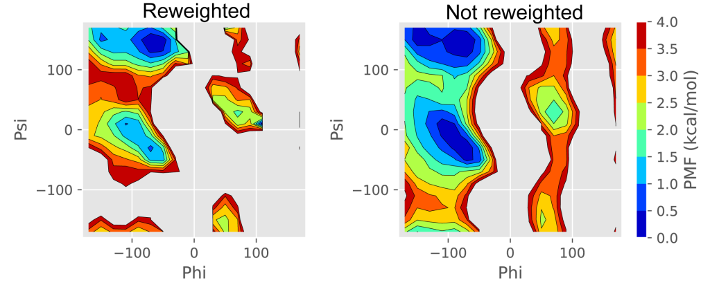
Figure 4. The reweighted and unreweighted free-energy landscapes of two dihedral angles of (Ala)3.
You can obtain the free-energy landscape without reweighting according to the following commands.
$ python ./calc_pmf_2d.py -t 300.0 -c 10.0 -n 1000000 --Xmin -180.0 --Xmax 180.0 --Xdel 20.0 --Ymin -180.0 --Ymax 180.0 --Ydel 20.0 --cv_file cv.dat --out_file out.dat --Xcyclic --Ycyclic --noreweightThe unreweighted free-energy landscape constructed from the obtained dihedral angles is shown in Figure 4. Due to the GaMD biases, the populations of the αR and C7ex conformations are overestimated, while the β/C5 conformation is underestimated. We can confirm that these overestimations and underestimations are modified in the above reweighting.
References
- Y. Miao, V. A. Feher, and J. A. McCammon. Gaussian Accelerated Molecular Dynamics: Unconstrained Enhanced Sampling and Free Energy Calculation. J. Chem. Theory Comput., 11, 3584–3595 (2015).
- Y. T. Pang, Y. Miao, Y. Wang, and J. A. McCammon. Gaussian Accelerated Molecular Dynamics in NAMD. J. Chem. Theory Comput., 13, 9–19 (2017).
- Y. Miao, W. Sinko, L. Pierce, D. Bucher, R. C. Walker, and J. A. McCammon. Improved Reweighting of Accelerated Molecular Dynamics Simulations for Free Energy Calculation. J. Chem. Theory Comput., 10, 2677–2689 (2014).
- D. Hamelberg, J. Mongan, and J. A. McCammon. Accelerated Molecular Dynamics: A Promising and Efficient Simulation Method for Biomolecules. J. Chem. Phys., 120, 11919–11929 (2004).
Written by Hiraku Oshima@RIKEN BDR
June 1, 2022