18.2 Coarse-grained MD simulation of DNA with the 3SPN.2C model
Contents
(This tutorial is for GENESIS v1.7.0 and later)
In the 3SPN.2C model [1], every nucleotide is represented by three coarse-grained particles, phosphate (P), sugar (S), and base (B). Here we show an example of simulating the partial melting and re-hybridization of a 50bp double-stranded DNA (dsDNA) with the 3SPN.2C model in GENESIS.
0. Preparations
0.1 Install necessary softwares
As introduced in tutorial 18.1, we use the GENESIS-CG-tool to generate CG MD files. In this tutorial we will use one script in the GENESIS-CG-tool to build CG DNA structure and topology from the nucleic acid sequence.
0.2 Download the files for this tutorial
Let’s download the tutorial file (tutorial19-18.2.zip). This tutorial consists of three steps: 1) system setup, 2) MD simulations (including two sub-steps), and 3) trajectory analysis.
# Download and unarchive the tutorial files
$ cd /home/user/GENESIS/Tutorials
$ unzip tutorial19-18.2.zip
$ cd tutorial-18.2
$ ls
01_setup 02.1_simulation_melting 02.2_simulation_hybridization 03_analysis
1. Setup
In this step, we are going to create the topology and coordinate files from a DNA sequence.
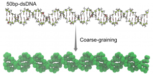
Coarse-graining of double stranded DNA.
Change to our working directory:
$ cd 01_setup
$ ls
dsDNA.fasta
This file dsDNA.fasta contains a randomly generated sequence for our 50-bp dsDNA. Use the cat command to have a look at its content:
$ cat dsDNA.fasta
> random sequence
GTCTTCGACGGGACCCGGTCTCGTCGACGACTGGACGGACCCCGCATAGC
We then use the following script in the GENESIS-CG-tool to build the atomistic structure and CG files for the dsDNA:
$ /home/user/genesis_cg_tool/tools/modeling/DNA_general/build_dna.jl -s dsDNA.fasta -C -o dsDNA
After running the command above, we will get some new files:
dsDNA.pdb: atomistic structure of the DNA;dsDNA_cg.topanddsDNA_cg.itp: CG topology files;dsDNA_cg.gro: CG coordinate file;dsDNA_cg.cif: CG PDB in the format of mmCIF.
Among these files, we have to modify dsDNA_cg.top a bit to apply the electrostatic interactions on DNA. Specifically, please make modifications or add the following two lines to dsDNA_cg.top:
[ cg_ele_chain_pairs ]
ON 1 - 2 : 1 - 2
The second line tells GENESIS to calculate electrostatic interactions between chain 1 to 2. As another example, “ON 1 - 3 : 4 - 6” means electrostatic interactions between chains 1 to 3 and chains 4 to 6. Please refer to the wiki-page of GENESIS-CG-tool for more information.
2. MD simulations
In this part, we are going to simulate the partial melting of the dsDNA (2.1), and then the re-hybridization (2.2), as shown in the following figure:
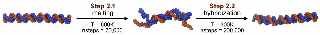
2.1 DNA melting
Let’s move to the working directory of the melting simulation:
$ cd 02.1_simulation_melting
$ ls
dna_md1.inp param/
The “param/” directory contains standard topology parameter files. The file “dna_md1.inp” is the control file for GENESIS to perform the MD simulation:
[INPUT]
grotopfile = dsDNA_cg.top
grocrdfile = dsDNA_cg.gro

[OUTPUT]
pdbfile = dna_md1_melt.pdb
dcdfile = dna_md1_melt.dcd
rstfile = dna_md1_melt.rst

[ENERGY]
forcefield            = RESIDCG
electrostatic         = CUTOFF
cg_cutoffdist_ele     = 52.0
cg_cutoffdist_DNAbp   = 18.0
cg_pairlistdist_ele   = 57.0
cg_pairlistdist_DNAbp = 23.0
cg_pairlistdist_exv   = 15.0
cg_sol_ionic_strength = 0.15

[DYNAMICS]
integrator      = VVER_CG
nsteps          = 20000
timestep        = 0.010
eneout_period   = 1000
crdout_period   = 1000
rstout_period   = 1000
nbupdate_period = 20

[CONSTRAINTS]
rigid_bond = NO

[ENSEMBLE]
ensemble    = NVT
tpcontrol   = LANGEVIN
temperature = 600
gamma_t     = 0.01

[BOUNDARY]
type = NOBC
Most of the options are the same as what we used for protein (see tutorial 18.1) except for the additional cutoff and pairlist distances for electrostatic and DNA base-pairing interactions.
Besides, here we set the temperature to 600K so that our DNA can be partially melted during the 20,000 MD steps.
Now let’s copy necessary files to the same directory:
$ cp ../01_setup/dsDNA_cg.top .
$ cp ../01_setup/dsDNA_cg.gro .
$ cp ../01_setup/dsDNA_cg.itp .
Then we can run the simulation with atdyn:
$ export OMP_NUM_THREADS=2
$ mpirun -np 4 /home/user/GENESIS/bin/atdyn dna_md1.inp > dna_md1_melt.log
The simulation finishes within a few minutes. We get these four new files:
dna_md1_melt.pdb: last structure of DNA in the simulation;dna_md1_melt.dcd: trajectory of DNA melting;dna_md1_melt.rst: MD restarting file;dna_md1_melt.log: GENESIS log file of the simulation.
There are two ways to see whether the DNA melted during the simulation. The first one is to see the “BASE_PAIR” energy from the dna_md1_melt.log file, whose value changed from -257.5075 kcal/mol to a value of ~-50 kcal/mol (might be different in your simulations). Another way is to see the structure of dna_md1_melt.pdb using softwares such as VMD. You can see the untangled DNA strands at the two ends.
Note that due to the randomness of the Langevin dynamics, the DNA may not melt enough in your simulations. In this case, you may have to increase the simulation length (“nsteps”) to let DNA melt. However, a more thoroughly melt DNA also takes much longer time to refold, and you may have to significantly increase the simulation steps in the next section to see the hybridization of DNA.
2.2 DNA hybridization
Let’s move on to refolding the double stranded DNA:
$ cd 02.2_simulation_hybridization
$ ls
dna_md2.inp param/
Again, “param/” is the directory for parameter files. Whereas “dna_md2.inp” is the control file for GENESIS:
[INPUT]
grotopfile = dsDNA_cg.top
grocrdfile = dsDNA_cg.gro
rstfile    = dna_md1_melt.rst

[OUTPUT]
pdbfile = dna_md2_hybrid.pdb
dcdfile = dna_md2_hybrid.dcd
rstfile = dna_md2_hybrid.rst

[ENERGY]
forcefield            = RESIDCG
electrostatic         = CUTOFF
cg_cutoffdist_ele     = 52.0
cg_cutoffdist_DNAbp   = 18.0
cg_pairlistdist_ele   = 57.0
cg_pairlistdist_DNAbp = 23.0
cg_pairlistdist_exv   = 15.0
cg_sol_ionic_strength = 0.15

[DYNAMICS]
integrator      = VVER_CG
nsteps          = 200000
timestep        = 0.010
eneout_period   = 1000
crdout_period   = 1000
rstout_period   = 1000
nbupdate_period = 20

[CONSTRAINTS]
rigid_bond = NO

[ENSEMBLE]
ensemble    = NVT
tpcontrol   = LANGEVIN
temperature = 300
gamma_t     = 0.01

[BOUNDARY]
type = NOBC
The main difference between this input file and the one in step 2.1 is that we changed the temperature to 300K, to simulate the hybridization of the dsDNA. We also want to use the partially melt DNA structure (from step 2.1) as the initial structure, therefore we set rstfile = dna_md1_melt.rst in the [INPUT] section.
Now let’s copy necessary files to this directory:
$ cp ../01_setup/dsDNA_cg.top .
$ cp ../01_setup/dsDNA_cg.gro .
$ cp ../01_setup/dsDNA_cg.itp .
$ cp ../02.1_simulation_melting/dna_md1_melt.rst .
Then we run the simulation:
$ export OMP_NUM_THREADS=2
$ mpirun -np 4 /home/user/GENESIS/bin/atdyn dna_md2.inp > dna_md2_hybrid.log
The simulation would take a few minutes on a laptop. After the simulation, we will get four new files:
dna_md2_hybrid.pdb: last structure of DNA in the simulation;dna_md2_hybrid.dcd: trajectory of DNA hybridization;dna_md2_hybrid.rst: MD restarting file;dna_md2_hybrid.log: GENESIS log file of the DNA hybridization simulation.
3. Analysis
Here we show how to compute RMSD from the trajectories we get in step 2.1 and 2.2.
$ cd 03_analysis
$ ls
rmsd_melt.inp   rmsd_hybrid.inp
The two “inp” files are the input files for GENESIS analysis tools. Let’s take a look at the “melt” one (the other one is similar):
[INPUT]
grotopfile = ../02.1_simulation_melting/dsDNA_cg.top
grocrdfile = ../02.1_simulation_melting/dsDNA_cg.gro

[OUTPUT]
rmsfile = run_melt.rms

[TRAJECTORY]
trjfile1 = ../02.1_simulation_melting/dna_md1_melt.dcd
md_step1 = 20000
mdout_period1 = 1000
ana_period1 = 1
trj_format = DCD
trj_type = COOR

[SELECTION]
group1 = all

[FITTING]
fitting_method = TR+ROT
fitting_atom = 1

[OPTION]
check_only = NO
The reference structure for the RMSD calculation is ../02.1_simulation_melting/dsDNA_cg.gro.
Let’s run GENESIS to get the RMSD:
/home/user/GENESIS/bin/crd_convert rmsd_melt.inp
/home/user/GENESIS/bin/crd_convert rmsd_hybrid.inp
We will get two new files containing the RMSD data:
$ ls
run_melt.rms
run_hybrid.rms

$ head run_melt.rms
  1   2.867
  2   3.045
  3   2.758
  4   2.770
  5   2.830
  6   2.671
  7   4.019
  8   6.358
  9   7.478
  10  8.370
Now you may use your favorite data-visualization tool to plot the time series of RMSD during the two MD simulations.
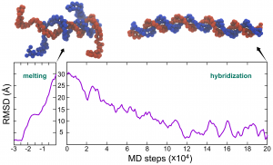
Time series of RMSD of dsDNA in the CG MD simulations of melting and hybridization.
A note on using VMD to visualize the DNA structure: the CG PDB files output by atdyn (dna_md1_melt.pdb and dna_md2_hybrid.pdb) write all the particles in one chain. To show the two DNA strands in different color, you can manually change the “chain ID” in these PDB files. Specifically in the current case, please change column 22 of atom 150-298 to “B”, and insert a new line “TER” before line 150. Then, you can set the coloring method to “Chain” in VMD.
References
[1] Freeman, G. S., Hinckley, D. M., Lequieu, J. P., Whitmer, J. K., de Pablo, J. J., 2014, J. Chem. Phy., 141 (16), 165103.Written by Cheng Tan@RIKEN Center for Computational Science, Computational Biophysics Research Team
October, 2021