17.1 Cryo-EM flexible fitting using a simulated map
Contents
Cryo-electron microscopy (Cryo-EM) is a powerful tool to determine three-dimensional structures of biomolecules at near atomic resolution. Flexible fitting has been widely utilized to model the atomic structure from the experimental density map [1]. One of the commonly used methods is the MD-based flexible fitting [2]. In GENESIS, c.c.-based flexible fitting is available in ATDYN and SPDYN [3]. In addition to the conventional methods, flexible fitting with the replica-exchange schemes (REUSfit [4]) or with the all-atom Go-model (MDfit [5]) is available in GENESIS. Here, we introduce a basic procedure to perform MD-based flexible fitting using a simulated density map with the GB/SA implicit solvent model (see also Tutorial 8.1) [6]. Experimental density map will be used in Tutorial 17.2 (under construction).
Preparation
First of all, let’s download the tutorial file (tutorial19-17.1.zip). In this tutorial, we additionally use the SITUS program package. If you have not installed it yet in your computer, please download and install the program in advance. Hereafter, we assume that the binary programs of SITUS ver. 3.1 are installed in /home/user/Situs_3.1/bin/. Since we use the CHARMM36m force field parameters, we make a symbolic link to the CHARMM toppar directory (see Tutorial 2.1).
# Put the tutorial file in the Works directory
$ cd ~/GENESIS_Tutorials-2019/Works
$ mv ~/Downloads/tutorial19-17.1.zip ./
$ unzip tutorial19-17.1.zip

# Clean up the directory
$ mv tutorial19-17.1.zip TRASH

# Update the README file
$ echo "tutorial-17.1: Cryo-EM flexible fitting using a simulated map" >> README

# Check the contents of Tutorial 17.1
$ cd tutorial-17.1
$ ln -s ../../Data/Parameters/toppar_c36_jul21 ./toppar
$ ln -s ../../Programs/genesis-1.7.1/bin ./bin
$ ls
1_emmap  3_minimize  5_analysis  toppar
2_build  4_fitting   bin
1. Making a simulated density map of the target state
Before dealing with a “real experimental” density map, let’s practice the flexible fitting using a “simulated” density map. Here, we employ the glucose/galactose binding protein (GGBP). Recently, the open and closed states of GGBP have been solved with the X-ray crystallography. We would like to create a target density map from the crystal structure of the open state (PDB: 2FW0), and carry out the flexible fitting from the closed state (PDB: 2FVY). Therefore, we know the “answer” of the fitting.
First, we download the PDB file of the open state (PDB: 2FW0), and create a processed PDB file that contains only protein heavy atoms by using VMD.
# Download PDB file of the open state of GGBP
$ cd 1_emmap
$ wget https://files.rcsb.org/download/2FW0.pdb

# Generate a new PDB file that contains protein heavy atoms
$ vmd -dispdev text 2FW0.pdb
vmd > set sel [atomselect top "protein and not hydrogen and not altloc B"]
vmd > $sel writepdb open.pdb
vmd > exit
To generate a synthetic density map from open.pdb, we use emmap_generator in the GENESIS analysis tool. We generate a control file INP using the “-h ctrl” option, and edit the file.
# Generate a control file of emmap_generator
$ ../bin/emmap_generator -h ctrl > INP
$ ls
2FW0.pdb  INP  open.pdb
We specify the following parameters in the control file. We create a map with the 5 Å resolution (sigma = 2.5 Å), where the file format is set to SITUS. The variable auto_margin makes a margin between the map edge and minimum or maximum coordinates of protein atoms according to the specified margin_size. Note that the original PDB file (2FW0.pdb) cannot be used as input in this tool.
# Control file of emmap_generator
#
[INPUT]
pdbfile       = open.pdb

[OUTPUT]
mapfile       = open.sit

[OPTION]
check_only    = NO        # (YES/NO)
allow_backup  = NO        # (YES/NO)
map_format    = SITUS     # (SITUS)
auto_margin   = YES       # (YES/NO)
margin_size_x = 20.0      # margin size
margin_size_y = 20.0      # margin size
margin_size_z = 20.0      # margin size
voxel_size    = 1.0       # voxel size
sigma         = 2.5       # resolution parameter
tolerance     = 0.001     # tolerance (0.001 = 0.1%)
After running emmap_generator for INP, let’s view the generated density map and open.pdb by using VMD. The following is an example to load the map file by the command line. This can be also done by using a mouse as follows [File > New Molecule > Browse > Select “open.sit” > Load].
# Generate synthetic EM density map (open.sit)
$ ../bin/emmap_generator INP > log
$ ls
2FW0.pdb  INP  log  open.pdb  open.sit

# Visualization by using VMD
$ vmd -situs ../1_emmap/open.sit
vmd > mol load pdb open.pdb
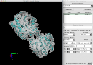
Figure 1. Comparison between the PDB and synthetic density map. Let’s change the representation of the density map by specifying “Wireframe” or by moving a seek bar of the “Isovalues”, which show the absolute value of the density data.
2. Building the initial structure
Second, we prepare the initial structure of the closed state (PDB: 2FVY). Again, we download the PDB file and create a processed PDB file that contains only protein heavy atoms:
# Download PDB file of the closed state of GGBP
$ cd ../2_build/
$ wget https://files.rcsb.org/download/2FVY.pdb
$ ls
2FVY.pdb

# Generate PDB file containing protein heavy atoms
$ vmd -dispdev text 2FVY.pdb
vmd > set sel [atomselect top "protein and not hydrogen and not altloc B"]
vmd > $sel writepdb proa.pdb
vmd > exit
$ ls
2FVY.pdb  proa.pdb
Let’s visualize proa.pdb and open.sit by using VMD. We can see that the position of the initial structure is significantly shifted from the target density. We have to fit the initial structure to the map as much as possible with a rigid docking protocol before the flexible fitting. For this purpose, we use the colores program in SITUS (for details, see here). We run the following command, where the resolution of 5 Å and 4 CPU cores are specified. It may take a few minutes for this calculation.
# Perform rigid docking using SITUS
$ /home/user/Situs_3.1/bin/colores ../1_emmap/open.sit proa.pdb -res 5 -nprocs 4
We obtained several PDB files, named col_best_00X.pdb. We should select the best model among them. The cross-correlation coefficient (c.c.) between the target and simulated densities is written in the header information of each PDB file. We see that col_best_001.pdb shows the best c.c., which means that this PDB is the best fitted model.
# Check the c.c. value in the obtained PDB files
$ ls col_*.pdb
col_best_001.pdb  col_best_003.pdb  col_best_005.pdb  col_best_007.pdb
col_best_002.pdb  col_best_004.pdb  col_best_006.pdb

$ grep "Unnormalized correlation coefficient:" col_*.pdb
col_best_001.pdb:REMARK Unnormalized correlation coefficient: 0.876832
col_best_002.pdb:REMARK Unnormalized correlation coefficient: 0.798847
col_best_003.pdb:REMARK Unnormalized correlation coefficient: 0.798821
col_best_004.pdb:REMARK Unnormalized correlation coefficient: 0.764940
col_best_005.pdb:REMARK Unnormalized correlation coefficient: 0.751088
col_best_006.pdb:REMARK Unnormalized correlation coefficient: 0.750453
col_best_007.pdb:REMARK Unnormalized correlation coefficient: 0.405601
Let’s compare col_best_001.pdb and open.sit by using VMD to check whether the protein is actually superimposed onto the map.
We use col_best_001.pdb as the initial coordinates of the flexible fitting. In order to use the CHARMM force field in the flexible fitting, we create PDB and PSF files with the all-atom model by using VMD (for details, see Tutorial 2.2):
$ vmd -dispdev text
vmd > package require psfgen
vmd > resetpsf
vmd > topology ../toppar/top_all36_prot.rtf
vmd > pdbalias residue HIS HSD
vmd > pdbalias atom ILE CD1 CD
vmd > segment PROA {pdb col_best_001.pdb}
vmd > coordpdb col_best_001.pdb PROA
vmd > guesscoord
vmd > writepdb closed.pdb
vmd > writepsf closed.psf
vmd > exit
We obtained closed.pdb and closed.psf. In addition to these files, we make a PDB file with the all-atom model for open.pdb, which will be used for the analysis of the RMSD with respect to the target state.
$ cd ../1_emmap
$ vmd -dispdev text
vmd > package require psfgen
vmd > resetpsf
vmd > topology ../toppar/top_all36_prot.rtf
vmd > pdbalias residue HIS HSD
vmd > pdbalias atom ILE CD1 CD
vmd > segment PROA {pdb open.pdb}
vmd > coordpdb open.pdb PROA
vmd > guesscoord
vmd > writepdb target.pdb
vmd > exit
3. Energy minimization
Before running the MD-based flexible fitting, energy minimization is usually needed to remove steric clashes in the initial structure. The control file is already contained in the directory. Here, we simply perform the energy minimization. We execute ATDYN for INP. After the calculation, min.dcd and min.rst are obtained.
# Perform energy minimization using 16 CPU cores
$ cd ../3_minimize
$ export OMP_NUM_THREADS=4
$ mpirun -np 4 ../bin/atdyn INP > log
$ ls
INP  log  min.dcd  min.rst
4. Flexible fitting
Then, we carry out the flexible fitting. The control file is already included in the directory.
# Change directory to run the simulation
$ cd ../4_fitting
$ ls
INP

# Take a look at the control file
$ less INP
The following shows the most important parts in the control file. You can recognize that the flexible fitting is a kind of “restrained MD simulation”, and most parameters are common with the conventional MD simulations. We apply the biasing potential on the protein heavy atoms, where the force constant of the bias is set to 5,000 kcal/mol. emfit_sigma is a resolution parameter, which is usually set to the half of the resolution of the target density map.
[INPUT]
topfile = ../toppar/top_all36_prot.rtf
parfile = ../toppar/par_all36m_prot.prm
pdbfile = ../2_build/closed.pdb
psffile = ../2_build/closed.psf
rstfile = ../3_minimize/min.rst

[SELECTION]
group1          = all and not hydrogen

[RESTRAINTS]
nfunctions      = 1
function1       = EM                  # apply restraints from EM density map
constant1       = 5000                # force constant in Ebias = k*(1 - c.c.)
select_index1   = 1                   # apply restraint force on protein heavy atoms

[EXPERIMENTS]
emfit           = YES                 # perform EM flexible fitting
emfit_target    = ../1_emmap/open.sit # target EM density map
emfit_sigma     = 2.5                 # half of the map resolution (5 A)
We execute ATDYN for INP. The following is an example to execute mpirun using 16 CPU cores:
# Perform flexible fitting
$ export OMP_NUM_THREADS=4
$ mpirun -np 4 ../bin/atdyn INP > log
$ ls
INP  log  run.dcd  run.pdb  run.rst
After the calculation, we obtain run.dcd, run.pdb, and run.rst, where the PDB file is the structure at 50 ps. The log file contains time courses of the energy and c.c. (Column 19: RESTR_CVS001). Let’s view the trajectory by using VMD. You can see that the structure is well fitted to the target density.
$ vmd -situs ../1_emmap/open.sit
vmd > mol load pdb ../2_build/closed.pdb psf ../2_build/closed.psf
vmd > mol addfile run.dcd
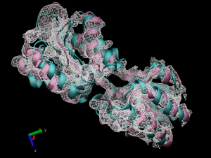 Figure 2. Comparison between the Initial (green) and fitted (red) structures.
5. Trajectory analysis
5.1 Cross-correlation coefficient and RMSD
First, we analyze the time courses of c.c., which can be easily obtained by using the following command. We select the value in the Column 19 (RESTR_CVS001) in the log file. You can see that the c.c. is successfully increased during the fitting.
# Change directory for analysis
$ cd ../5_analysis

# Analyze time courses of c.c.
$ grep "INFO:" ../4_fitting/log | awk '{print $3, $19}' | grep -v "RESTR" > cc.log
$ less cc.log
Second, we analyze the RMSD with respect to the target structure, because we know what should be the correct “answer” in this flexible fitting. Here, we use rmsd_analysis in the GENESIS analysis tool set, as in Tutorial 3.3. We use target.pdb as reference coordinates. Please, confirm that the number of atoms as well as the order of atoms in target.pdb and closed.pdb are identical to each other, otherwise the atom selection or RMSD calculation cannot be done correctly.
# Analysis of the RMSD
$ ../bin/rmsd_analysis INP
$ ls
INP  cc.log  output.rms
We obtain output.rms. Let us plot the RMSD and c.c. by using gnuplot. We can see that the RMSD with respect to the target state is quickly decreased as the c.c. increased. The c.c. is eventually converged in 50 ps.
# Plot the c.c. and RMSD data
$ gnuplot
gnuplot> set encoding iso
gnuplot> set y2tics
gnuplot> set ytics nomirror
gnuplot> set xlabel "Time (ps)"
gnuplot> set ylabel "c.c."
gnuplot> set y2label "RMSD (\305)"
gnuplot> unset key
gnuplot> plot 'cc.log' u ($0/5):2 w l,'output.rms' u ($0/5):2 w l axis x1y2
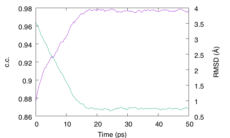
Figure 3. Time courses of c.c. (purple line) and Cα RMSD with respect to the target structure (green line).
5.2 MolProbity score
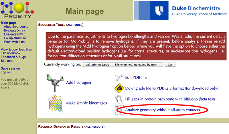
Finally, we evaluate the quality of the obtained structure. One of the commonly used criteria is the MolProbity score [7], which represents how good the structure is as a protein. It can be computed with the GUI server. Let’s access to the MolProbity Server, and upload run.pdb obtained from the flexible fitting.
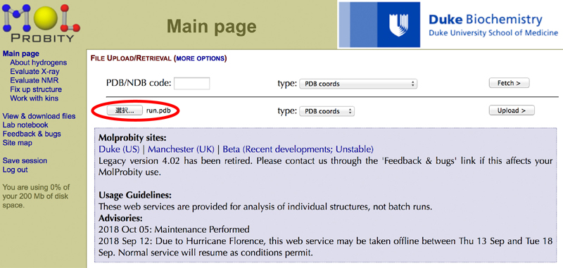
After the process, we click “Analyze geometry without all-atom contacts”.
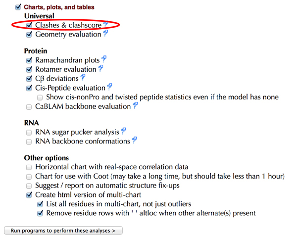
Confirm that the “Clashes & clashscore” for Charts, plots, and tables is checked.
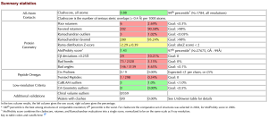
We found that the MolProbity score of run.pdb was 1.43.
References
- F. Tama et al., J. Mol. Biol., 337, 985-999 (2004).
- M. Orzechowski and F. Tama, Biophys. J., 95, 5692-5705 (2008).
- T. Mori et al., Structure, 27, 161-174.e3 (2019).
- O. Miyashita et al., J. Comput. Chem., 38, 1447-1461 (2017).
- P. Whitford et al., PNAS, 108, 18943-18948 (2011).
- A. Onufriev et al., Proteins, 55, 383-394 (2004).
- V. B. Chen et al., Acta Cryst., D66, 12-21 (2010).
Written by Takaharu Mori@RIKEN Theoretical molecular science laboratory
April. 21, 2022