16.1. QM/MM calculation of alanine-tripeptide in water
Contents
- Preparation
- 1. MD simulations of alanine tripeptide
- 2. Generation of a cluster system
- 3. Setting up a QM/MM calculation
- 4. Geometry optimization of an alanine tripeptide
- 5. Harmonic vibrational analysis of an amide group of Ala3
- References
- Appendix A. The template input file for Gaussian (gaussian.com)
- Appendix B. The script to run Gaussian (runGau.sh)
In this tutorial, we illustrate how to perform QM/MM calculations in GENESIS. QM/MM method is a multiscale approach, first proposed in seminal papers by Warshel and Karplus [1] and Warshel and Levitt [2] and, which treats a chemically important region by the electronic structure theory (QM) and the surrounding environment by a molecular mechanics force field (MM). The method was recently implemented into GENESIS [3]. Here, we illustrate how to perform QM/MM calculations to obtain the structure and the vibrational spectrum of alanine tripeptide (Ala3) in solution.
This tutorial requires Gaussian 09 or later for QM calculations.
Preparation
Let’s download the tutorial file (tutorial-16.1.tar.gz ). This tutorial consists of five steps. In step 1, we carry out classical MD simulations of Ala3 in water. Then, in step 2, we show how to extract a snapshot structure and create a cluster system from MD data using qmmm_generator. A system consisting of Ala3 and water molecules within 20.0 Å of Ala3 will be created. After these preparations, we perform a QM/MM calculation using GENESIS with GAUSSIAN in step 3. The input files for GENESIS and GAUSSIAN, as well as script files to run/control the jobs are explained. Geometry optimization and vibrational analysis of an amide group will be presented in step 4 and 5, respectively. Since we use the CHARMM36m force field parameters, we make a symbolic link to the CHARMM toppar directory (see Tutorial 2.1).
$ cd Tutorials
$ mv ~/Downloads/tutorial-16.1.tar.gz ./
$ tar -xvzf tutorial-16.1.tar.gz
$ cd tutorial-16.1
$ ln -s ../../Others/CHARMM/toppar ./
$ ls
0_charmm-gui/ 1_md/      2_setup/      3_qmmm/       4_qmmm-min/   5_qmmm-vib/   toppar/
1. MD simulations of alanine tripeptide
Let’s first look into a folder 0_charmm-gui/
$ cd 0_charmm-gui
$ ls
ala3.pdb   step2_solvator.pdb   step2_solvator.psf
A representative structure of Ala3 is given in ala3.pdb (see Tutorial 3.2).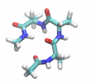
From ala3.pdb, we have generated psf and pdb files of Ala3 in water using Solvator of CHARMM-GUI. You can access Solvator in the left menu of the top page by clicking “Input Generator” and then “Solvator”. The procedure to create a water box is quite intuitive and straightforward. We just note that,
- Upload ala3.pdb
- Terminal group patching was ACE for first and CT3 for last
- Set the waterbox size to X: 50, Y:50, Z:50
- Ions not included (check off “Include Ions” and click “Calculate number of ions”)
The resulting psf and pdb files, step2_solvator.psf and step2_solvator.pdb, are used for the following MD simulations.
$ cd ../1_md
$ ls
run.sh*   step1.1.inp  step1.2.inp  step1.3.inp  step1.4.inp
step1.*.inp are input files to carry out,
- step1.1: Minimization for 2000 steps
- step1.2: NVT simulation for 50 ps with restraint to heavy atoms of Ala3
- step1.3: NPT simulation for 50 ps with restraint to heavy atoms of Ala3
- step1.4: NPT simulation for 50 ps without restaint
In fact, these calculations are the same as those in Tutorial 3.2, where you find more details about input options.
run.sh is a script to run GENESIS.
#!/bin/bash

spdyn=../../../bin/spdyn

export OMP_NUM_THREADS=2
mpirun -np 8 $spdyn step1.1.inp >& log1.1
mpirun -np 8 $spdyn step1.2.inp >& log1.2
mpirun -np 8 $spdyn step1.3.inp >& log1.3
mpirun -np 8 $spdyn step1.4.inp >& log1.4
Configure the number of OMP threads and/or MPI processes for your system. Then type,
$ chmod +x run.sh
$ ./run.sh
2. Generation of a cluster system
Let’s look into the trajectory of step1.4, step1.4.dcd, using VMD,
$ vmd -psf ../0_charmm-gui/step2_solvator.psf -dcd step1.4.dcd
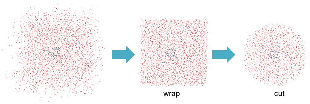
You can see that many water molecules have diffused out of the simulation box. To create a cluster system for QM/MM calculations, these molecules first need to be wrapped back in the simulation box. Furthermore, we often want to cut molecules that are far away (say, 20.0 Å) from the QM region. “qmmm_generator” is a tool to help this wrap & cut procedure.
$ cd ../2_setup
$ ls
qmmm_generator.inp   run.sh*
“qmmm_generator.inp” is an input file for qmmm_generator. The content is shown in the following.
[INPUT] section[INPUT] psffile = ../0_charmm-gui/step2_solvator.psf reffile = ../0_charmm-gui/step2_solvator.pdb
The psf and pdb files are specified in psffile and reffile, respectively. They need to be consistent with dcd files specified in the [TRAJECTORY] section below.
[OUTPUT]
qmmm_crdfile   = snapshot{}.crd
qmmm_psffile   = snapshot{}.psf
qmmm_pdbfile   = snapshot{}.pdb
Coordinate, psf, and pdb files of generated systems are specified in qmmm_crdfile, qmmm_psffile, and qmmm_pdbfile, respectively. The curvy brackets “{}” will be replaced by a snapshot ID in the program. Note that the number of atoms may change after the cutting procedure, so that not only pdb/crd but also psf are generated for each snapshot.
[TRAJECTORY]
trjfile1       = ../1_md/step1.4.dcd
md_step1       = 25000
mdout_period1  = 500
ana_period1    = 500
trj_type       = COOR+BOX
trj_natom      = 0
The dcd file is specified by trjfile1. There are 50 snapshots in step1.4.dcd with nsteps = 25000 and crdout_period = 500. In other words, the trajectory was printed every 1 ps up to 50 ps. md_step1 and mdout_period1 are the same as nstep and crdout_period. ana_period1 is the frequency of snapshot structures used for the analysis. trj_type = COOR+BOX means the dcd file includes the information of both coordinates and a box size. trj_natom = 0 takes the number of atoms from a reffile of [INPUT]. For more details about this section, see FAQ.
[SELECTION]
group1         = segid:PROA
group2         = segid:PROA or (segid:PROA around_mol:20.0)
group1 selects Ala3. group2 selects Ala3 and water molecules that are within 20.0 Å of Ala3. Note that the selector command, A around_mol:r, selects a molecule if one of its atoms is within r Å of any atom of A. Also, A around_mol:r selects the molecules around A, but NOT A itself. Therefore, we need to use A or (A around_mol:r) to select a QM/MM system.
[OPTION]
origin_atom_index   = 1
qmmm_atom_index     = 2
frame_number        = 10:10:50
coord_format        = CHARMM
reconcile_num_atoms = NO
check_only          = NO
origin_atom_index and qmmm_atom_index specify the origin of the system and atoms to be included in a QM/MM system, respectively. In this example, the center of mass of group1 (= Ala3) is set to the origin, and the atoms in group2 (= Ala3 and water molecules around Ala3) are selected for a QM/MM system. The snapshot ID can be specified through frame_number in two ways: either by directly writing the ID number with camma spearator or by a format of startID:stride:endID. 10:10:50 means starting from 10, every 10 frame up to 50. It is equivalent to frame_number = 10, 20, 30, 40, 50. coord_format specifies the output format; currently only CHARMM crd file is available. If reconcile_num_atoms = YES, the program makes the number of atoms as much similar as possible among all snapshots.
qmmm_generator is invoked by run.sh,
#!/bin/bash

# Generate QM/MM systems
../../bin/qmmm_generator qmmm_generator.inp >& qmmm_generator.out
Now, type
$ chmod +x run.sh
$ ./run.sh
When successful, you will find snapshotID.psf, .pdb, .crd, for ID = 10, 20, 30, 40, and 50 . You may visually check the created system using VMD,
$ vmd snapshot50.pdb -psf snapshot50.psf
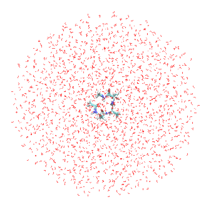
Hereafter, we will use snapshot 50 for QM/MM calculations; the same calculations are readily possible for other snapshot structures.
Although we don’t attempt here, it is often useful to perform minimization at the MM level prior to QM/MM.
3. Setting up a QM/MM calculation
Let’s move into a folder of QM/MM calculations:
$ cd 3_qmmm
$ ls
gaussian.com    qmmm.inp    runGau.sh*    script.sh*
qmmm.inp is a control file for GENESIS. Here, we just calculate the QM/MM energy for given input coordinates by setting nstep = 0 in the [MINIMIZE] section.
gaussian.com and runGau.sh are a template input file for Gaussian and a script to invoke Gaussian from GENESIS, respectively. script.sh is a script to run GENESIS. We will look into these files in the following.
(a) The control file for GENESIS
qmmm.inp sets options needed for treating a cluster system and QM/MM as the energy function. Important options are described below.
[ENERGY]
forcefield       = CHARMM
electrostatic    = CUTOFF
switchdist       = 16.0    # switch distance
cutoffdist       = 18.0    # cutoff distance
pairlistdist     = 19.5    # pair-list distance
vdw_force_switch = YES

[BOUNDARY]
type = NOBC
In [ENERGY], electrostatic is set to CUTOFF, and switch/cutoff/pairlist distances are set to be longer than in the case of PME. Accordingly, type in [BOUNDARY] is set to NOBC.
[QMMM]
qmtyp              = gaussian            (1)
qmcnt              = gaussian.com        (2)
qmexe              = runGau.sh           (3)
qmatm_select_index = 1                   (4)
workdir            = qmmm_min            (5)
basename           = job                 (6)
qmsave_period      = 1                   (7)
qmmaxtrial         = 1                   (8)
exclude_charge     = group               (9)

[SELECTION]
group1  = atomno:1-14                    (10)
(1) qmtyp specifies a program for QM calculations. Here, we choose Gaussian.
(2) (3) qmcnt is the name of a template file to generate input files for Gaussian and qmexe is the name of a script file to invoke Gaussian. The procedure of QM/MM calculations is sketched in the figure below.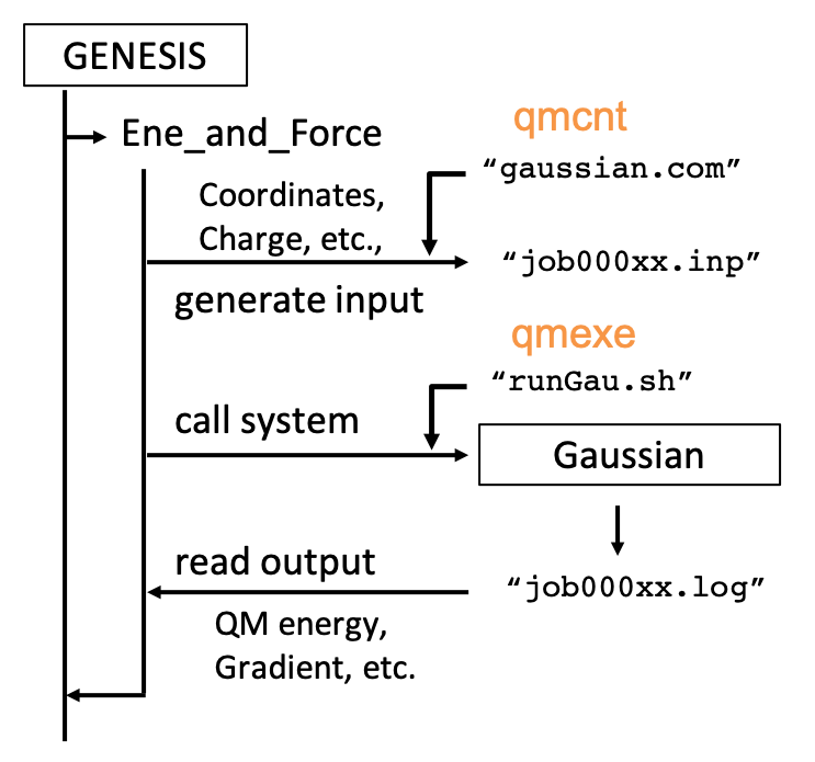
(4) (10) qmatm_select_index = 1 specifies QM atoms as group1 in [SELECTION]. In this example, the first 14 atoms (i.e., ALA1 except for the carboxylic group) are selected. The blue shaded region is the QM atoms in a figure below. GENESIS automatically sets a link hydrogen atom between CA and C.

NOTES:
1. Make sure that the psf has correct information not only for MM atoms but also for QM atoms, because the covalent bond capped by the link hydrogen is detected based on an entry for chemical bonds in psf.
2. Make sure that the covalent bond at the QM – MM boundary is a single bond, since only one hydrogen is added to a terminus QM atom. It may result in error if you cut double bonds or aromatic bonds.
(5) workdir is the name of directory where the files for QM calculations are generated.
(6) basename is a basename of QM files. The file name becomes jobXXXX.{inp, log}, where XXXX is a step number.
(7) qmsave_period = 1 sets a period to save the files of QM calculations.
(8) qmmaxtrial sets the maximum number to repeat QM calculations upon its failure. It sometimes happens that QM jobs fail unexpectedly due to SCF unconvergence, network trouble, etc. In such case, GENESIS repeats the same calculation for the number of times specified here.
(9) exclude_charge sets a scheme to remove the MM charge in the vicinity of link hydrogens. GROUP removes the MM charge of the same group in the CHARMM force field.
(b) The template file for Gaussian
Important keywords of gaussisan.com are listed below.
%chk=gaussian.chk               (1)
...
scf(conver=8) iop(4/5=100) NoSymm Charge Force Prop=(Field,Read) pop=mk        (2)
...
#coordinate#       (3)
#charge#           (4)
#elec_field#       (5)
(1) The name of a checkpoint file must be “gaussian.chk”. Never remove or change this line.
(2) These are keywords for Gaussian.
scf(conver=8) runs the SCF calculation with a convergence criterion of 10-8 Hartree. The threshold is reduced by 2 upon restart.
iop(4/5=100) is a directive to read molecular orbitals (MO) from a checkpoint file if present.
NoSymm prevents reorientation of axis.
Charge reads MM coordinates and charges.
Force calculates the force in addition to the energy.
Prop=(Field,Read) calculates the electric field at given positions.
pop=mk calculates the ESP charge of QM atoms obtained by fitting the electrostatic potential generated by the electron density to that of atomic charges.
(3), (4), (5) are replaced by coordinates of QM atoms, coordinates and charge of MM atoms, and coordinates of MM atoms, respectively, in the program.
See Appendix for further details on the input options.
(c) The script file to run Gaussian
The first part of runGau.sh is shown below. The text in red must be properly set by users,
export g09root=/path/to/gaussian        (1)
export GAUSS_EXEDIR=$g09root/g09
export GAUSS_EXEBIN=$g09root/g09/g09
export PATH=$PATH:$GAUSS_EXEDIR
export LD_LIBRARY_PATH=${GAUSS_EXEDIR}:${LD_LIBRARY_PATH}

# --- Set the path for a scratch folder ---
scratch=/scr/$USER                      (2)
# (optional)
# --- Set a chkpoint file to read initial MOs ---
#initialchk='../path/to/initial.chk'    (3)
(1) Set a path to a folder where Gaussian is installed.
(2) Set a path to a scratch folder. If your machine has a fast, local disk equipped, it is better to use it as a scratch folder. Guassian (and most QM programs) writes a large intermediate file, so that the speed of disk access may significantly affect the performance.
(3) Optionally, set a checkpoint file to read initial MO.
Note that GENESIS calls the script in the following way,
$ runGau.sh job.com job.log 0
where the first and second arguements are the name of input and output files of Gaussian, respectively, and the third one is the step number in MINIMIZE or MD. It is a good practice to test the script with the above command and see if Gaussian runs propery.
(d) Running QM/MM in GENESIS
Finally, script.sh is a file to run GENESIS.
export QM_NUM_THREADS=16     (1)
export OMP_NUM_THREADS=16    (2)

# 1) Open MPI
#
mpirun -np 1 --map-by node:pe=${QM_NUM_THREADS} atdyn qmmm.inp >& qmmm.out    (3)

# 2) Intel MPI
#
# mpirun -np 1 -ppn 1 atdyn qmmm.inp >& qmmm.out    (4)
(1) (2) QM_NUM_THREADS and OMP_NUM_THREADS set the number of thread for Gaussian jobs and GENESIS, respectively.
(3) In case of OpenMPI, --map-by node:pe=${QM_NUM_THREADS} is needed to have a child process (= QM jobs) to run in thread parallel.
(4) In case of Intel MPI, a simple command works.
You may now run the job by typing,
$ chmod +x script.sh runGau.sh
$ ./script.sh
Upon successful run, you will find the following message in the output file (qmmm.out) showing that the atoms of number 1 to 14 are selected as QM atoms,
Setup_QMMM> Setup QM region
QM assignment info
1  PROA 1 ALA CAY CT3 assigned to QM atom 1  of element: C 6
2  PROA 1 ALA HY1 HA3 assigned to QM atom 2  of element: H 1
3  PROA 1 ALA HY2 HA3 assigned to QM atom 3  of element: H 1
4  PROA 1 ALA HY3 HA3 assigned to QM atom 4  of element: H 1
5  PROA 1 ALA CY  C   assigned to QM atom 5  of element: C 6
6  PROA 1 ALA OY  O   assigned to QM atom 6  of element: O 8
7  PROA 1 ALA N   NH1 assigned to QM atom 7  of element: N 7
8  PROA 1 ALA HN  H   assigned to QM atom 8  of element: H 1
9  PROA 1 ALA CA  CT1 assigned to QM atom 9  of element: C 6
10 PROA 1 ALA HA  HB1 assigned to QM atom 10 of element: H 1
11 PROA 1 ALA CB  CT3 assigned to QM atom 11 of element: C 6
12 PROA 1 ALA HB1 HA3 assigned to QM atom 12 of element: H 1
13 PROA 1 ALA HB2 HA3 assigned to QM atom 13 of element: H 1
14 PROA 1 ALA HB3 HA3 assigned to QM atom 14 of element: H 1
number of QM atoms = 14
Subsequently, the information on link atoms are printed,
Generate_LinkAtoms> QM-MM interface info. Link hydrogen is set between:
      [ QM atom ]   - [ MM atom ]
9 PROA 1 ALA CA CT1 - 15 PROA 1 ALA C C
                      16 PROA 1 ALA O O excluded

number of link atoms = 1
The QM – MM boundary is set between CA(9) and C(15) of ALA1. The MM charge O(16) is also excluded in QM calculations, because C(15) and O(16) belongs to the same group in the CHARMM force field. In the end of the output, you will find an entry for QM energy,
$ grep INFO qmmm.out |awk '{print $14}'
QM
-180636.9869
The input/output files of Gaussian are found in a qmmm_min.0 folder,
$ ls qmmm_min.0
gaussian.chk  min00000.Fchk  min00000.inp  min00000.log
To summarize, you need to prepare four files to run QM/MM calculations:
- a control file for GENESIS
- a template to generate input files of a QM program
- a script to invoke QM jobs
- a script to run GENESIS
Example files for other QM programs (e.g., Q-Chem, TeraChem, DFTB+) are found in our github repository.
4. Geometry optimization of an alanine tripeptide
Let’s calculate the geometry of Ala3 using the QM/MM method.
$ cd 4_qmmm-min/
$ ls
gaussian.com@ minimize.gpi qmmm_min.inp runGau.sh@ script.sh*
Note that gaussian.com and runGau.sh are symblic links to the previous ones in 3_qmmm. The control file for GENESIS is qmmm_min.inp. It is similar to 3_qmmm/qmmm.inp except for options in the [MINIMIZE] section.
[MINIMIZE]
method              = LBFGS      (1)
nsteps              = 300  # number of steps
eneout_period       = 1    # energy output period
crdout_period       = 5    # coordinates output period
rstout_period       = 5    # restart output period
nbupdate_period     = 10   # non-bonded pair-list update period
fixatm_select_index = 2          (2)
macro               = yes        (3)

[SELECTION]
group1 = atomno:1-14
group2 = not (segid:PROA or (segid:PROA around_mol:15.0))  (4)
(1) LBFGS is an efficient algorithm to energy-minimize the structure, and is recommended for a tight optimization prior to vibrational analyses.
(2) (4) fixatm_select_index = 2 fix the atoms specified in group2 of [SELECTION]. In this case, water molecules that are distant from Ala3 by more than 15.0 Å are fixed. The fix is necessary to prevent water molecules from reorientation at the edge of the cluster.
(3) macro = yes invokes a macro/micro-iteration method. In this scheme, the optimization is carried out in two loops. Both QM and MM atoms are relaxed in the outer loop, while only MM atoms are relaxed with QM atoms fixed in the inner loop. During the inner loop, the QM atoms are represented by ESP charges and QM calculations are not required. Thus, it leads to a significant speed up of the calculation.
Run the program using script.sh,
$ chmod +x script.sh
$ ./script.sh
The convergence of optimization is checked by the magnitude of root-mean-square gradient (RMSG) and the maximum gradient (MAXG). The tolerence by default is set to be 0.36 and 0.54 kcal mol-1 Å-1. These values can be changed by tol_rmsg and tol_maxg in the [MINIMIZE] section.
In this example, the iteration will be around 100 cycles. You will see a message in the end of the log file when the convergence is reached.
>>>>> STOP: RMSG and MAXG becomes sufficiently small
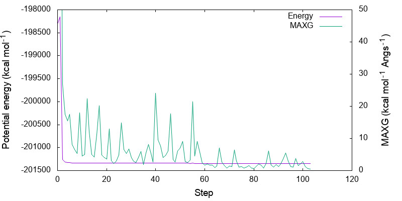
Let us plot the variation of the potential energy and MAXG as a function of step number.
> grep INFO qmmm_min.out >& minimize.log
> gnuplot minimize.gpi
Because the variation in the potential energy is huge in the first few steps, you may adjust the range of y-axis by modifying minimize.gpi,
> vi minimize.gpi
...
set yrange  [-201343:-201338]...

> gnuplot minimize.gpi
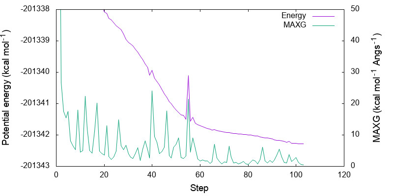
You can see that both energy and MAXG become small along the step. Note that the energy is converged with an accuracy of 1 kcal mol-1 around the 60-th step, while it takes 40 more steps to converge MAXG. A similar behavior is often seen for geometric parameters as well.
When you plot the figure, the energy values and the convergence behavior may be different from the above. This is because the result is dependent on the initial structure, and the last snapshot of MD trajectory you used may be different from that of the example.
5. Harmonic vibrational analysis of an amide group of Ala3
Let’s carry out the harmonic vibrational analysis of Ala3 using the QM/MM method. In this calculation, the Hessian matrix of a partial system is calculated by numerical differentiations of the gradient. It requires the gradient at 6N + 1 grid points, where N is the number of atoms for the vibrational analysis. The calculation is parallelized over the grid points, i.e., multiple QM calculations run simultaneously for different grid points. We also use the MO obtained for the equilibrium geometry as the initial MO to speed up the SCF convergence.
$ cd ../5_qmmm-vib/
$ ls
gaussian.com@ qmmm_vib.inp runGau.sh script.sh*
Note that gaussian.com is a symblic link to the previous one in 3_qmmm. The control file for GENESIS is qmmm_vib.inp.
[INPUT]
topfile = ../toppar/top_all36_prot.rtf     # topology file
parfile = ../toppar/par_all36m_prot.prm    # parameter file
strfile = ../toppar/toppar_water_ions.str  # stream file
psffile = ../2_setup/snapshot50.psf        # protein structure file
crdfile = ../2_setup/snapshot50.crd        # CRD file
reffile = ../2_setup/snapshot50.pdb        # PDB file
rstfile = ../4_qmmm-min/qmmm_min.rst    (1)

[OUTPUT]
minfofile = qmmm_vib.minfo              (2)
(1) restarts from the optimized structure obtained in the last step.
(2) minfofile is a file where the harmonic normal modes and frequencies will be written.
Instead of [MINIMIZE], we now have a new section, [VIBRATION].
[VIBRATION]
runmode             = HARM      (1)
nreplica            = 4         (2)
vibatm_select_index = 2         (3)
output_minfo_atm    = 3         (4)

[SELECTION]
group1  = atomno:1-14
group2  = atomno:5-8            (5)
group3  = segid:PROA            (6)
(1) sets the calculation to the harmonic analysis.
(2) specifies the number of QM (=MPI) processes to run in parallel.
(3) and (5) sets the target atoms for vibrational calculations to the first amide group (CY, OY, N, and HN) of Ala3.
(4) and (6) sets the atoms to print in a minfofile.
runGau.sh is the same as the previous one except that we use the initial MO of the last run,
# --- Set a chkpoint file to read initial MOs ---
initialchk='../4_qmmm-min/qmmm_mini.0/gaussian.chk'
In script.sh, we specify 4 MPI processes. This must be the same as nreplica in [VIBRATION] section. Assuming that you have 2 nodes each with 16-core CPU,
export  QM_NUM_THREADS=8
export OMP_NUM_THREADS=8

# 1) Open MPI
#
mpirun -np 4 --map-by node:pe=${QM_NUM_THREADS} $GENESIS qmmm_vib.inp >& qmmm_vib.out
# 2) Intel MPI
#
#mpirun -np 4 -ppn 2 $GENESIS qmmm_vib.inp >& qmmm_vib.out
With this setting, you will have 2 MPI processes running in each node. You may run the program using script.sh,
$ chmod +x script.sh
$ ./script.sh
In the output file (qmmm_vib.out), you can check the atoms selected for vibrational analysis
Enter vibrational analysis

  Cartesian coordinates of atoms for vib. analysis
     1          5 PROA      1 ALA    CY           -4.0454035711      6.0518032659     -1.0542278637
     2          6 PROA      1 ALA    OY           -3.6124748284      6.0503734927      0.1129067982
     3          7 PROA      1 ALA    N            -3.2838770224      5.8998076018     -2.1586664849
     4          8 PROA      1 ALA    HN           -3.7438296522      6.0476346883     -3.0591784947
Then, we see the iteration of QM/MM calculations over the grid points,
Generate Hessian matrix by num. diff. of gradients
Loop over atoms
Done for 0 input replicaID = 1 energy = -201342.288637
Done for 1 CY -X replicaID = 3
Done for 1 CY +Y replicaID = 4
Done for 1 CY +X replicaID = 2
Done for 1 CY +Z replicaID = 2
...
Done for 4 HN -Z replicaID = 1

RMSD of the gradient at the input geometry = 0.175137D+00 [kcal mol-1 Angs-1]
It is a good practice to make sure that the gradient at the input geometry (= equilibrium geometry) is sufficiently small. You will see a warning message if the gradient is large. In that case, check if the input geometry (rstfile) is correct, if the preceding minimization is converged, and so on. Then, the harmonic frequencies (in cm-1), infrared (IR) intensity (in km mol-1), and normal displacement vectors are printed,
  Harmonic frequencies and normal displacement vectors
          mode             1           2           3           4           5
          omega        180.6477    288.7726    363.8458    428.9706    701.4632
         IR int.        11.9316      9.3777      0.3900      9.5531     78.8291
         1   CY   X      0.0166      0.0788     -0.0464      0.2521     -0.0362
         1   CY   Y      0.2860      0.0002     -0.2796      0.0123     -0.4383
         1   CY   Z     -0.0297     -0.3755      0.0315      0.3513     -0.0605
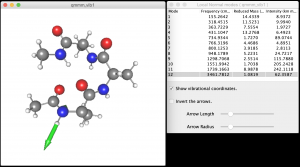
The minfofile (qmmm_vib.minfo) can be visulalized using JSindo . Below is a screenshot of JSindo that shows the N-H stretching mode of an amide group.
Try a calcluation with all water molecules fixed. For such calculation, you need to change
group2 = not segid:PROA
in qmmm_min.inp. How does the vibrational frequency change?
References
- A. Warshel and M. Karplus, J. Am. Chem. Soc., 94, 5612-5625 (1972).
- A. Warshel and M. Levitt, J. Mol. Biol., 103, 227-249 (1976).
- K. Yagi, K. Yamada, C. Kobayashi, and Y. Sugita, J. Chem. Theory Comput. 15, 1924-1938 (2019).
Appendix A. The template input file for Gaussian (gaussian.com)
The template file for Gaussian is the following.
%chk=gaussian.chk                         .... (1)
%NProcShared=8                            .... (2)
%mem=1gb                                  .... (3)
#P b3lyp/cc-pVDZ EmpiricalDispersion=GD3  .... (4)
scf(conver=8) iop(4/5=100) NoSymm Charge  .... (5)
Force Prop=(Field,Read) pop=mk            .... (6)
                                          .... (7)
Gaussian run for QMMM in genesis          .... (8)
                                          .... (9)
0 1                                       .... (10)
#coordinate#                              .... (11)
#charge#                                  .... (12)
#elec_field#                              .... (13)
(1) specifies the name of a check point file. Don’t change this line unless you are sure!
(2) specifies the number of CPU threads. This line is overwritten to match $QM_NUM_THREADS by runGau.sh (see below).
(3) specifies the amount of memory used by Gaussian. “1gb” means 1 giga-byte. We can also use “mb” for mega-byte. That is, “1000mb” is a synonym of “1gb”. Note that the memory here is only for one Gaussian job. Don’t forget to leave some room for GENESIS. Also, pay attention to the number of QM jobs that runs in a node. The maximum amount of memory specified here would be,
maxMemory = (mem_of_system – mem_for_OS) / (num_of_proc_per_node) – mem_for_GENESIS
(4) – (6): These are options to control QM calculations in Gaussian. Visit the Gaussian website for further details.
b3lyp/cc-pVDZ uses B3LYP functions for DFT and cc-pVDZ for the basis sets
EmpiricalDispersion=GD3 uses D3 dispersion correction
scf(conver=8) sets SCF convergence to 10-8 Hartree.
iop(4/5=100) restarts SCF if the previous MO is present in a checkpoint file (=gaussian.chk)
Nosymm keeps the XYZ orientation of a system
Charge sets MM point charges in QM calculations
Force calculates the gradient of the energy
Prop=(field, read) calculates the electric field applied to MM point charges
pop=mk calculates ESP charges for QM atoms. This is required when macro = yes in [MINIMIZE].
(7) a blank line to set the end of options.
(8) a title line. This can be anything.
(9) a blank line to set the end of a title.
(10) specifies charge and spin multiplicity. Note that the former is the charge of a QM subsystem, not of the whole system. Multiplicity is 2s+1, where s is the spin of a QM subsystem.
(11)-(13) These directives are replaced with the coordinates of QM atoms and MM atoms.
Appendix B. The script to run Gaussian (runGau.sh)
#!/bin/bash
# -----------------------------------------------
# Settings for Gaussian09
#
# --- Set the path for Gaussian ---
export g09root=/usr/local/gaussian      ... (1)
export GAUSS_EXEDIR=$g09root/g09
export GAUSS_EXEBIN=$g09root/g09/g09
export PATH=$PATH:$GAUSS_EXEDIR
export LD_LIBRARY_PATH=${GAUSS_EXEDIR}:${LD_LIBRARY_PATH}

# --- Set the path for a scratch folder ---
scratch=./    ... (2)

# (optional)
# --- Set a chkpoint file to read initial MOs ---
#initialchk='../initial.chk'  ... (3)

QMINP=$1 ...(4)
QMOUT=$2
NSTEP=$3
MOL=${QMINP%.*}

# Initial MO
if [ $NSTEP -eq 0 ] && [ -n "${initialchk}" ] && [ -e ${initialchk} ]; then
   cp ${initialchk} gaussian.chk  ... (5)
fi

# Scratch folder settings
export GAUSS_SCRDIR=$scratch/$(mktemp -u $MOL.XXXX)  ... (6)
mkdir -p ${GAUSS_SCRDIR}

# SMP parallel setting
if [ -z "$QM_NUM_THREADS" ] && [ "${QM_NUM_THREADS:-A}" = "${QM_NUM_THREADS-A}" ]; then
    QM_NUM_THREADS=$OMP_NUM_THREADS  ... (7)
fi
TMP=$(mktemp tmp.XXXX)
echo "%NprocShared=${QM_NUM_THREADS}" >> $TMP
grep -v -i nproc $QMINP >> $TMP ... (8)
mv $TMP $QMINP

# Now exe g09 and create a formatted chk file
(time $GAUSS_EXEBIN < $QMINP) > ${QMOUT} 2>&1      ... (9)
formchk gaussian.chk gaussian.Fchk >& /dev/null

# Remove unnecessary folder
rm -rf ${GAUSS_SCRDIR}   ... (11)
(1) sets the path for Gaussian.
(2) sets the path for scratch files.
(3) modify to use existing check point file for restarting SCF.
(4) sets the input arguments to variables.
(5) copy the saved check point file, which contains the initial MO, to gaussian.chk. Note that this line is executed only for the first step ($NSTEP == 0).
(6) sets $GAUSS_SCRDIR to a temporary folder in $scratch. Gaussian uses this variable for a scratch folder.
(7) checks whether or not $QM_NUM_THREADS is set. If not, it defaults to $OMP_NUM_THREADS.
(8) modifies $QMINP so that %NprocShared equals to $QM_NUM_THREADS.
(9) executes Gaussian, and then generates a formatted checkpoint file (gaussian.Fchk). GENESIS retrieves the QM energy, gradient, and so on, from the log file ($QMOUT) and Fchk file.
(10) removes $GAUSS_SCRDIR. One may add other post processes here, for example, extracting quantities written in the log files. Note that $QMINP, $QMOUT, gaussian.Fchk are removed by GENESIS after reading the QM information if mod(NSTEP/qmsave_period) != 0.