8.2 MD simulation of TSPO in the implicit membrane model
Contents
In this tutorial, we simulate the translocator protein (TSPO) in the IMM1 implicit membrane model. The IMM1 model was originally developed by T. Lazaridis [1], and is available in the CHARMM program package. Recently, we have introduced IMM1 into GENESIS.
Preparation
First of all, parameter files for the EEF1/IMM1 implicit solvent model are needed, which are currently available in CHARMM. Please download the CHARMM program package in advance (installation is not required). Then, we make the eef1 directory in the ./Data/Parameters directory and copy the CHARMM C19 parameter and topology files for the EEF1/IMM1 model (solver.inp, toph19_eef1.1.inp, and param19_eef1.1.inp) from CHARMM. Here, we assume that the users downloaded CHARMM in the ~/Downloads directory. The EEF1 parameter files are found in the support/aspara directory.
# Copy the EEF1 parameter files from CHARMM
$ cd ~/GENESIS_Tutorials-2022/Data/Parameters
$ mkdir eef1
$ cd ./eef1
$ cp ~/Downloads/charmm/support/aspara/solvpar.inp ./
$ cp ~/Downloads/charmm/support/aspara/toph19_eef1.1.inp ./
$ cp ~/Downloads/charmm/support/aspara/param19_eef1.1.inp ./
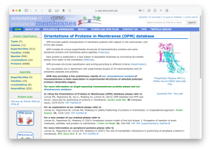
We will simulate the translocator protein (TSPO) in the IMM1 implicit membrane model, whose PDBID is 4RYO. In MD simulations of membrane proteins, the initial orientation and position of the protein relative to the membrane plane are important. The “OPM database” is one of the useful resources that provide optimal orientation and position of membrane proteins. Let’s access the website.
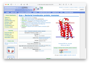
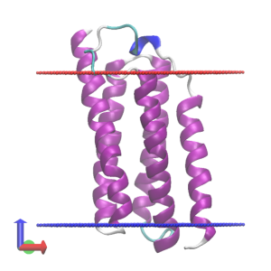
Let’s search for PDBID: 4RYO in the search window. Then you will see a page displaying the optimal orientation and hydrophobic thickness of 4RYO. The optimal thickness is shown as 31.4 Å. You can download the PDB structure with the optimal orientation. We would like to put the downloaded PDB file in the Data directory.
# Download the "reoriented PDB structure" of TSPO
$ cd ~/GENESIS_Tutorials-2022/Data/
$ mkdir OPM
$ cd OPM
$ wget https://opm-assets.storage.googleapis.com/pdb/4ryo.pdb

# Check the structure using VMD
$ vmd 4ryo.pdb
Now, let’s download the tutorial file (tutorial22-8.2.zip). The tutorial consists of five steps: 1) system setup, 2) energy minimization, 3) equilibration, 4) production run, and 5) trajectory analysis. Control files for GENESIS are already included in the file.
# Download the tutorial file
$ cd ~/GENESIS_Tutorials-2022/Works
$ mv ~/Downloads/tutorial22-8.2.zip ./
$ unzip tutorial22-8.2.zip

# Clean up the directory
$ mv tutorial22-8.2.zip TRASH

# Let's take a note
$ echo "tutorial-8.2: MD simulation of TSPO in the implicit membrane" >> README

# Check the contents of Tutorial 8.2
$ cd tutorial-8.2
$ ln -s ../../Programs/genesis-2.0.0/bin ./bin
$ ln -s ../../Data/Parameters/eef1 ./
$ ls
1_setup  2_minimize  3_equilibrate  4_production  5_analysis  bin  eef1
1. Setup
We first build the input PDB and PSF files using psfgen. The script is already contained in the 1_setup directory. Here, proa.pdb and proa.psf are obtained. In addition, we make “memb.pdb” that contains the dummy atoms representing the membrane plane.
# Change directory for the system setup
$ cd 1_setup
$ ln -s ../../../Data/OPM/4ryo.pdb ./
$ ls
4ryo.pdb  build.tcl

# Make PDB and PSF files
$ vmd -e build.tcl
$ ls
4ryo.pdb  build.tcl  proa.pdb  proa.psf  tmp.pdb

# Make a PDB file that represents membrane
$ grep "DUM" 4ryo.pdb > memb.pdb
2. Minimization
To use the IMM1 implicit membrane model in GENESIS, we specify eef1file in the [INPUT] section, and “implicit_solvent = IMM1” and “imm1_memb_thick” in the [ENERGY] section. Here, we specify “imm1_memb_thick = 31.4” according to the OPM database. For the other options for IMM1, please see the GENESIS user manual.
# Change directory for energy minimization
$ cd ../2_minimize
$ less INP
[INPUT]
parfile  = ../eef1/param19_eef1.1.inp
topfile  = ../eef1/toph19_eef1.1.inp
eef1file = ../eef1/solvpar.inp
pdbfile  = ../1_setup/proa.pdb
psffile  = ../1_setup/proa.psf

[ENERGY]
forcefield       = CHARMM19 # [CHARMM19]
electrostatic    = CUTOFF   # [CUTOFF]
switchdist       = 18.0     # switch distance
cutoffdist       = 20.0     # cutoff distance
pairlistdist     = 22.0     # pair-list distance
implicit_solvent = IMM1     # [IMM1]
imm1_memb_thick  = 31.4     # membrane thickness

[BOUNDARY]
type             = NOBC     # [NOBC]
Then, we execute ATDYN. The following is an example command using 4 CPU cores.
# Run ATDYN
$ export OMP_NUM_THREADS=1
$ mpirun -np 4 ../bin/atdyn INP > log
3. Equilibration
In the equilibration run, we carry out a 10-ps MD simulation at 298.15K with positional restraints on the Cα atoms. The equations of motion are integrated with the velocity Verlet algorithm with the time step of 2 fs, where the SHAKE and RATTLE algorithms are used for bond constraint. The [ENERGY] section is the same as the previous energy minimization. We use the Langevin thermostat to consider the random effects of the solvent on the solute atoms.
# Change directory for equilibration
$ cd ../3_equilibrate
$ less INP
[ENSEMBLE]
ensemble         = NVT       # [NVE,NVT]
tpcontrol        = LANGEVIN  # [NO,BERENDSEN,BUSSI,LANGEVIN]
temperature      = 298.15    # initial and target temperature (K)
Let’s execute ATDYN. In the log file, the solvation free energy is shown in the 14th column (SOLVATION).
# Run ATDYN
$ mpirun -np 4 ../bin/atdyn INP > log
4. Production run
In the production run, we carry out a 100-ps MD simulation without any restraints. The control file is almost identical to the previous equilibration run. The simulation time is extended, and the positional restraint is now turned off.
# Change directory for production run
$ cd ../4_production

# Run ATDYN
$ mpirun -np 4 ../bin/atdyn INP > log

# Check the MD trajectory
$ vmd -f ../1_setup/memb.pdb -f ../1_setup/proa.pdb -psf ../1_setup/proa.psf -dcd md.dcd
5. Trajectory analysis
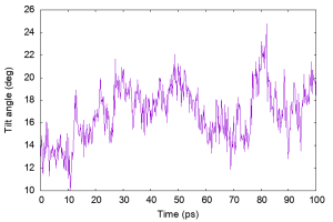
Helix tilt angle
We demonstrate the analysis of the helix tilt angle using the “tilt_analysis” tool in GENESIS, which computes the angle between the principal axis of a specified transmembrane (TM) helix and the z-axis (the bilayer normal). In the example, we analyze the residues 5–24.
# Analyze the helix tilt angle
$ cd ../5_analysis/
$ cd ./helix_tilt
$ ls
INP

$ ../../bin/tilt_analysis INP
$ ls
INP  output.out
Let’s plot the results.
References
- T. Lazaridis, Proteins, 52, 176-192 (2003).
Written by Takaharu Mori@RIKEN Theoretical molecular science laboratory
June 17, 2022