7.4 All-atom Go-model for the molten globule simulation of RNase-H protein
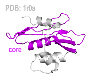
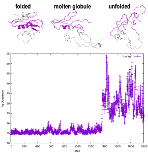
In the tutorial 7.3, we used Cα Go-model, which coarse-graining each amino acid residue as one bead. Here, we use another coarse-grained model, all atom Go (AA Go) model which can describe higher-order effect such as side chain interaction of protein [1]. With this model, we are going to simulate the unfolding of RNase H protein from HIV-1 (RNase-H), and observe molten globule state of the molecule [2].
You can download the tutorial files and please unpack the zip into a working directory.
# download the tutorial file
$ cd /home/user/GENESIS/Tutorials
$ mv ~/Downloads/tutorial22-7.4.zip ./
$ unzip tutorial22-7.4.zip
$ cd tutorial-7.4
$ ls
1_setup 2_production 3_analysis
- system setup
- production run
- trajectory analysis
1. Setup the system
Firstly, you need to install SMOG2 [3-5], a software to generate coarse-grained model of biomolecules, on your local machine. You can download both source codes and user manual of SMOG2 from its website. Installation and configuration of SMOG2 is described from page 3 to page 5 on the user manual. Before installation of SMOG2, you have to verify an availability of some prerequisites such as Perl, Perl Data Language (PDL), and various modules. You can install these modules by using yum (Red-Hat), apt-get (Debian), and so on depending your operating system. Here are examples in Ubuntu:
$ sudo apt-get install -y perl # Perl
$ sudo apt-get install -y libxml-parser-perl libxml-simple-perl libxml-perl \
                          libxml-sax-expatxs-perl libxml-validate-perl \
                          libxml-validator-schema-perl # XML module
$ sudo apt-get install -y libsub-exporter-perl libexporter-tiny-perl \
                          libexporter-autoclean-perl libexporter-cluster-perl \
                          libexporter-declare-perl libexporter-easy-perl \
                          libexporter-lite-perl libexporter-renaming-perl \
                          libexporter-tidy-perl # Exporter module
$ sudo apt-get install -y pdl libpdl-stats-perl # PDL
$ sudo apt-get install -y libgetopt-long-descriptive-perl # Getopt module
$ sudo apt-get install -y libscalar-util-numeric-perl \
                          libscalar-list-utils-perl # Scalar module
Once you have installed SMOG2 on your machine, you can generate input files for MD simulation, a coordinate file (.gro) and a topology/parameter file (.top), from X-ray crystallographic structure by using SMOG2. The X-ray structure of HIV-1 reverse transcriptase, containing RNase-H, is available from the RCSB Protein Data Bank (PDB). You can download the PDB file (PDB ID: 1r0a) on a web browser, or with running the following commands:
# change to the setup directory
$ cd /path/to/1_setup

# download the PDB file (PDB ID: 1r0a)
$ wget https://files.rcsb.org/download/1r0a.pdb
You have to extract RNase-H from the PDB file by trimming off the other part:
# extract RNase-H from 1r0a.pdb
$ head -n6198 1r0a.pdb | tail -n932 > 1r0a_mod.pdb

# add END statement which is necessary to run SMOG2
$ echo END >> 1r0a_mod.pdb
Then we perform SMOG2 with 1r0a_mod.pdb:
# adjust format of the input PDB file
$ smog_adjustPDB -i 1r0a_mod.pdb # adjusted.pdb file will be generated as an output

# Generate structure-based AA-Go model by using SMOG2
$ smog2 -i adjusted.pdb -AA > setup.log
After running SMOG2, you can see four output files (smog.gro, .top, .ndx, and .contacts). Among them, you will use .gro and .top files in the following MD simulation.
2. Production run
Just same as Tutorial 7.3, we are going to perform a production run without energy minimization or equilibration.
The following commands perform a 1.0 x 10^7 steps (20 ns) simulation with atdyn:
# change to the production run directory
$ cd /path/to/2_production

# set the number of OpenMP threads
$ export OMP_NUM_THREADS=1

# perform production run with atdyn by using 8 MPI processors
$ mpirun 8 -np 8 atdyn run.inp | tee run.out
The control file run.inp contains several sections, such as [INPUT], [OUTPUT], and [ENERGY], where we can specify the control parameters for the simulation. In the [INPUT] section, we set the file names for the initial coordinate file (.gro) and the topology/parameter file (.top)(see section 4.1 of the GENESIS manual for an explanation of each input file).
In the [OUTPUT] section, output filenames are set. Atdyn does not create any output file unless we explicitly specify their names. Here in our example, the restart file (.rst) and the binary trajectory file (.dcd) are set (see section 4.2 of the GENESIS manual for an explanation of each output file).
In the [ENERGY] section, we specify the parameters related to the energy and force evaluation. AAGO is the name for the AA Go-model in GENESIS. We set large values for the cutoff (switchdist=45, cutoffdist=50, pairlistdist=55) to perform a nearly “non-cutoff” simulation. The user can consider a different value to balance computational efficiency and accuracy, in case of large biomolecular systems.
The [DYNAMICS] section sets up the parameters for the MD engine of atdyn. In this tutorial, time step can be set to 2 fs without SHAKE constraints, by specifying rigid_bond=NO in the [CONSTRAINTS] section.
In the [ENSEMBLE] section, the LANGEVIN thermostat is chosen for an isothermal simulation with the friction constant of 0.1 ps-1.
Finally, in the [BOUNDARY] section, we set the boundary condition for the system, which is no boundary condition (NOBC) here.
[INPUT]
grotopfile     = ../1_setup/smog.top # topology/parameter file
grocrdfile     = ../1_setup/smog.gro # coordinate file (equivalent to PDB file)

[OUTPUT]
dcdfile        = run.dcd # DCD trajectory file
rstfile        = run.rst # restart file

[ENERGY]
forcefield     = AAGO
electrostatic  = CUTOFF
switchdist     = 45.0 # this will be ignored
cutoffdist     = 50.0 # cutoff distance
pairlistdist   = 55.0 # pair-list cutoff distance

[DYNAMICS]
integrator     = VVER # [LEAP, VVER]
nsteps         = 10000000 # number of MD steps
timestep       = 0.002 # time step (ps)
eneout_period  = 5000 # energy output period
crdout_period  = 5000 # coordinate output period
rstout_period  = 10000000 # restart output period

[CONSTRAINTS]
rigid_bond     = NO

[ENSEMBLE]
ensemble       = NVT # [NVE, NVT, NPT]
tpcontrol      = LANGEVIN # thermostat
temperature    = 112.5 # target temperature (K)
gamma_t        = 0.1 # friction (ps-1) # in [LANGEVIN]

[BOUNDARY]
type           = NOBC # [PBC, NOBC]
3. Trajectory analysis
As an example for the analysis, we use the rg_analysis, which calculates a radius of gyration (Rg) for each snapshot in the trajectory. You can perform rg_analysis with following commands:
# change to the analysis directory
$ cd /path/to/3_analysis/

# set the number of OpenMP threads
$ export OMP_NUM_THREADS=1

# perform rg_anlaysis
$ rg_analysis run.inp | tee run.out
The control file for the Rg calculation is shown below:
[INPUT]
grotopfile     = ../1_setup/smog.top # topology/parameter file
grocrdfile     = ../1_setup/smog.gro # coordinate file

[OUTPUT]
rgfile         = run.rg # Rg file

[TRAJECTORY]
trjfile1       = ../2_production/run.dcd # trajectory file
md_step1       = 10000000 # number of MD steps
mdout_period1  = 5000 # MD output period
ana_period1    = 5000 # analysis period
repeat1        = 1 # repeat times

trj_format     = DCD # (PDB/DCD)
trj_type       = COOR+BOX # (COOR/COOR+BOX)
trj_natom      = 0 # (0:uses atom count in PDB)

[SELECTION]
group1         = all # selection group 1

[OPTION]
check_only     = NO # (YES/NO)
allow_backup   = NO # (YES/NO)
analysis_atom  = 1 # atom group
mass_weighted  = YES
In the [TRAJECTORY] section, we set the input trajectory files as trjfile1=../2_production/run.dcd.
In the [SELECTION] section, we define a group (group1) of all atoms in the model which are used for the Rg calculation. Finally, the Rg output file (rgfile=run.rg) is set in the [OUTPUT] section.
By running rg_analysis, we get an Rg file (run.rg). The first column of this file is the indices of time step, and the second column is the Rg values in the unit of Angstrom. We can visualize it with programs such as gnuplot:
$ gnuplot
gnuplot> set xlabel “Step”
gnuplot> set ylabel “Rg [Angstrom]”
gnuplot> plot “run.rg” w lp
References
- L. Wang et al., J. Chem. Phys., 128, 235103 (2008).
- S. Yadahalli and S. Gosavi, Phys. Chem. Chem. Phys., 19, 9164-9173 (2017).
- J. K. Noel et al., PLoS Comput. Biol., 12, e1004794 (2016).
- P. C. Whitford et al., Proteins: Structure, Function, Bioinformatics, 75, 430-441 (2009).
- J. K. Noel et al., J. Phys. Chem. B 116, 8692-8702 (2012).
Written By Mao Oide @ RIKEN Theoretical molecular science laboratory
June 18, 2022