7.3 Dual-basin Go model for the open-to-close motions of Ribose Binding Protein
Contents
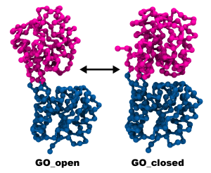
Conformational transitions in proteins play an important role in biological processes, many proteins undergo transitions between two (or more) conformations due to the binding of a ligand. In Tutorial 7.1 we learned to perform a coarse-grained simulation using the Karanicolas and Brooks Go (KB Go) model. There, it was assumed that the protein has a single stable conformation around its native folded state. In order to describe transitions between two conformations, single-basin (SB) potentials can be mixed into a dual-basin (DB) potential.
In this tutorial, we will learn how to setup and perform a dual-basin KB Go simulation for the open to closed motion of the ribose binding protein (RBP). The potential form is general and can be expanded to more than two basins (referred to as multi-basin, or MB, Go potentials).
Here, we use the exponential macroscopic mixing scheme as shown in the following equation [1,2]:
\( \displaystyle \exp\left(-\frac{1}{k_\mathrm{B}T_\mathrm{mix}}E\left(\mathbf{R}\right) \right)=\exp\left(-\frac{1}{k_\mathrm{B}T_\mathrm{mix}}\left(V_\mathrm{Open}\left(\mathbf{R}\right)+C\right)\right)+\exp\left(-\frac{1}{k_\mathrm{B}T_\mathrm{mix}}V_\mathrm{Closed}\left(\mathbf{R}\right)\right) \)
where \( \displaystyle k_\mathrm{B}\) is the Boltzmann constant and \( \displaystyle V_\mathrm{Open}\) and \( \displaystyle V_\mathrm{Closed}\) are the SB potentials of the open and closed structures, respectively. \( \displaystyle C\) and \( \displaystyle T_\mathrm{mix}\) are system-dependent parameters representing the basin’s relative energy and the barrier height, respectively. The parts of the SB potentials that are mixed in the DB potential are only the nonbonded native contacts. The rest of the terms are taken as averages or assigned some generic potential. The KB Go potential form is described in Ref. [3,4].
Let’s start by downloading the tutorial file tutorial22-7.3, extracting it, and verifying the contents of the directories:
# Download the tutorial file and confirm its content
$ cd /home/user/GENESIS/Tutorials
$ mv ~/Downloads/tutorial22-7.3.zip ./
$ unzip tutorial22-7.3.zip
$ cd tutorial22-7.3
$ ls
1_setup 2_simulation 3_analysis 4_mbar input_files output_files
The tutorial consists of four sections:
- Setup
- MD simulation
- Analysis
- Estimating mixing parameters using MBAR analysis
Input files which will be used frequently will be placed in the input_files directory. The directory output_files contains output files for all the tutorial steps so users can perform any step in the tutorial without depending on previous steps.
1. Setup
In this section, we will obtain the structures of the two conformations of RBP, create a KB Go coarse-grained model of them and obtain their KB Go potential files.
# Change directory
$ cd 1_setup
$ ls
1.1_get_pdb 1.2_get_sbgo 1.3_edit_sbgo 1.4_get_dbgo
1.1 Obtaining pdb files and editing them for further processing
We will download the protein structures from RCSB Protein Data Bank and use the VMD script pdb_write_chain.tcl to edit the structures:
# Change directory
$ cd 1.1_get_pdb

# Download the pdb files for open and closed conformations
$ wget http://www.rcsb.org/pdb/files/1urp.pdb
$ wget http://www.rcsb.org/pdb/files/2dri.pdb
$ ls *pdb
1urp.pdb 2dri.pdb

# Use the following script to clean the pdb files so that they will contain only chain A of the protein
$ vmd -dispdev text -e pdb_write_chain.tcl -args 1urp.pdb A
$ ls
$ ls *pdb
1urp_A.pdb 1urp.pdb 2dri_A.pdb 2dri.pdb
1.2 Obtaining KB Go structure and parameter files
We will use the MMTSB web server to create the CG structures and the KB Go potential files. Upload the edited files 1urp_A.pdb and 2dri_A.pdb to the server and create your KB Go-model files. Please refer to tutorial 7.1 for a detailed description of the usage of MMTSB server.
You will get a tarball file for each structure. Download and extract the files:
# Change directory
$ cd ../1.2_get_sbgo/

# Extract the tarball file
$ tar xvf ~/Downloads/1urp_A.tar
$ tar xvf ~/Downloads/2dri_A.tar
$ ls *1urp_A*
GO_1urp_A.param GO_1urp_A.pdb GO_1urp_A.Qdetails GO_1urp_A.Qlist GO_1urp_A.seq GO_1urp_A.top
The .pdb files contain the Cα structures, .param files are KB Go potential files, and .top files are CHRAMM-type topology files.
1.3 Creating .psf files and editing the KB Go .pdb files
We will use the VMD script edit_sbgo.tcl which does the following:
- reads the .pdb file obtained from MMTSB and renames residues from “ALA” to G1, G2, G3…
- aligns the center of mass with the origin.
- creates a .psf file using psfgen plugin in VMD (reads the .top and .pdb files obtained from MMTSB).
# Change directory
$ cd ../1.3_edit_sbgo/

# Run the script
$ vmd -dispdev text -e edit_sbgo.tcl -args ../1.2_get_sbgo/GO_1urp_A.pdb open
$ vmd -dispdev text -e edit_sbgo.tcl -args ../1.2_get_sbgo/GO_2dri_A.pdb closed
$ ls GO*
GO_closed.pdb GO_closed.psf GO_open.pdb GO_open.psf
The script also renamed the .pdb file to GO_open.pdb and GO_closed.pdb (and wrote the respective .psf files in the same names).
Let’s open the .pdb files in VMD and inspect their structures:
1.4 Creating a Dual-basin Go parameter file
Finally, we will mix the two single-basin (SB) parameter files to create a dual-basin (DB) potential parameter file. We will use two scripts:
pdb_kbgo_insert_resname.tcl, which will replace the G1, G2, G3,… residue names in the CG .pdb file into their original residue names required for creating the DB parameters file. The script requires the CG and the all-atom (AA) .pdb files as input.DB_grotop.plwhich creates the DB parameter file. The script requires CG .pdb files and SB .param files as input.
We will use the script run.sh to run the two scripts. Please confirm the contents of the script and see how to run it.
# Change directory
$ cd ../1.4_get_dbgo
$ ls
DB_grotop.pl pdb_kbgo_insert_resname.tcl run.sh

# Run the script
./run.sh
The scripts created the .grotop DB parameter file GO_open_closed_DB.grotop, let’s look at its content:
...
[ multicontact ]
4   252 2 1 9.79594800e-01 1.37571698e+01
5   35  2 1 4.59301800e-01 7.89473730e+00
6   36  2 1 4.75761400e-01 1.26628551e+01
7   46  2 1 7.13832500e-01 5.21756306e+00
7   50  2 1 7.33994400e-01 1.07868750e+01
8   38  2 1 5.16426600e-01 4.84627490e+00
...
239 263 2 1 6.75579000e-01 5.99921794e+00
243 263 2 1 7.83529100e-01 4.86581418e+00
2   252 2 2 9.61301700e-01 6.48675854e+00
3   57  2 2 7.01887500e-01 1.21176380e+01
4   60  2 2 5.00989600e-01 1.24774620e+01
5   61  2 2 5.05904000e-01 9.36764128e+00
7   37  2 2 4.82519700e-01 1.23629983e+01
12  16  2 2 7.66817600e-01 6.05881902e+00
...

[ pairs ]
1 33 2 6.40807600e-01 2.36451438e+00
2 32 2 5.54960300e-01 5.39343750e+00
2 33 2 6.02866050e-01 1.24115536e+01
2 59 2 7.03373200e-01 3.28296514e+00
3 33 2 4.57910450e-01 3.67379258e+00
3 35 2 6.95549300e-01 6.76133354e+00
3 59 2 6.08667550e-01 1.24115536e+01
3 60 2 7.62771950e-01 1.24115536e+01
4 32 2 6.73748350e-01 1.02592517e+01
...
Here we show only the parts which are exclusive to the DB potential. The [ multicontact ] field lists nonbonded interactions which are unique to each basin, where columns 1 and 2 are residue names, column 4 is the basin number (1 or 2), and column 5 and 6 are the parameters \( \displaystyle \sigma_\mathrm{ij}\) and \( \displaystyle \epsilon_\mathrm{ij}\), which represent the residue-pair distance in the native structure and the force constant, respectively. Here, basin 1 represents the open conformation and basin 2 represents the closed conformation, as they were listed in that order when we executed the DB_grotop.pl script. The [ pairs ] field lists the nonbonded interactions which are common to both basins where the parameters \( \displaystyle \sigma_\mathrm{ij}\) and \( \displaystyle \epsilon_\mathrm{ij}\) were taken as their averages between the two basins.
Now that we have created the structure and parameters files, we will copy them to a single directory:
# Copy files
$ cp GO_open_closed_DB.grotop ../../input_files/
$ cp ../1.3_edit_sbgo/GO_*.p* ../../input_files/

# Go to directory and confirm its content
$ cd ../../input_files/
$ ls
GO_closed.pdb GO_closed.psf GO_open_closed_DB.grotop GO_open.pdb GO_open.psf
Now we are ready to run the DB Go simulation.
2. MD simulation
Here we will simulate the open to closed motion of RBP using the DB Go potential that we just prepared.
# Change directory
$ cd ../2_simulation
$ ls
run_db.inp
GO_open_closed_DB.grotop is the GENESIS input file for running the DB Go simulation. Let’s look at it’s content:
[INPUT]
grotopfile  = ../input_files/GO_DB.grotop      # topology file
psffile     = ../input_files/GO_open.psf       # structure file
pdbfile     = ../input_files/GO_open.pdb       # .pdb coordinate file

[OUTPUT]
dcdfile     = run_db.dcd                       # .dcd trajectory file
rstfile     = run_db.rst                       # restart file

[ENERGY]
forcefield      = KBGO                         # name of force field
electrostatic   = CUTOFF                       # [CUTOFF/PME]
switchdist      = 19.9                         # switch distance
cutoffdist      = 20.0                         # cutoff distance
pairlistdist    = 50.0                         # pair-list cutoff distance
water_model     = NONE                         # no waters in KBGo
num_basins      = 2                            # number of basins
mix_temperature = 4500                         # Tf
basinenergy1    = -1.12                        # C
basinenergy2    = 0                            # should be set to zero

[DYNAMICS]
integrator      = VVER                         # [LEAP/VVER]
nsteps          = 100000                       # number of MD steps
timestep        = 0.020                        # timestep (ps)
eneout_period   = 10000                        # energy output period
rstout_period   = 10000                        # restart output period
crdout_period   = 10000                        # .dcd output period
nbupdate_period = 10                           # nonbonded output period
stoptr_period   = 1                            # frequency of removing trans'/rot'

[CONSTRAINTS]
rigid_bond      = YES                          # constraints all bonds
fast_water      = NO                           # no water
shake_tolerance = 1.0e-6                       # tolerance (Angstrom)

[ENSEMBLE]
ensemble        = NVT                          # [NVE/NVT/NPT]
tpcontrol       = LANGEVIN                     # thermostat
temperature     = 260                          # temperature of the simulation (K)
gamma_t         = 0.001                        # thermostat friction

[BOUNDARY]
type            = NOBC                         # no boundary conditions
In the [INPUT] section, we specify the DB parameter file name in grotopfile and the structure and initial coordinates in psffile and pdbfile, respectively. Note that we start the simulation with the open structure (GO_open.psf and GO_open.pdb), but since there will be transitions between the open and closed conformations, if the simulations are converged, we expect to obtain a similar structural ensemble if we start from the closed conformation.
In the [ENERGY] section, we set the potential to KBGO with num_basins = 2. We must specify the DB parameters \( \displaystyle C\) and \( \displaystyle T_\mathrm{mix}\) (mix_tgemperature and basinenergy1, respectively). Note that these parameters change from system to system and must be tuned in order to obtain an appropriate sampling of DB mixing. In section 4 we show how to efficiently determine those parameters using MBAR analysis method.
We run the simulations for 100,000 steps (nsteps). Note that this is a very short time, which was set for the purpose of the tutorial only. In order to obtain a reasonable sampling you will need to run your simulation for longer. We have prepared a separate trajectory running 25,000,000 steps in the output_files directory, on which we will demonstrate our analyses.
Now, let’s run the simulation:
# Set the number of OpenMP threads
$ export OMP_NUM_THREADS=1

# Perform a simulation using atdyn by using 8 MPI processes
$ mpirun -np 8 /path/to/atdyn run_db.inp | tee run_db.out
The simulation should take less than a minute. Please confirm that you obtained the following output files:
$ ls
run_db.dcd run_db.inp run_db.out run_db.rst
3. Analysis
We will now perform basic analyses of our DB simulation trajectory to characterize the transitions between the open and closed basins. We will perform our analysis on the longer trajectory which is in output_files/2_simulation_long.
The analysis procedures are found in the 3_analysis directory:
# Change directory
$ cd ../3_analysis
$ ls
3.1_dRMS 3.2_PMF_1D 3.3_PMF_2D 3.4_Keq
3.1 dRMS
We will use the distance root-mean-square displacement (dRMS) as a reaction coordinate for quantifying the similarity of the simulation frames to the open or closed conformations. dRMS is calculated between atom pairs which satisfy initial criteria according to the following equation [5]:
\( \displaystyle dRMS=\sqrt{\frac{1}{N_{contact}}\sum_{i\neq{}j\in{}contacts}\left[d\left(x_i^A,x_j^A\right)-d\left(x_i^B,x_j^B\right)\right]^2} \),where \( \displaystyle N_{contact}\) is the number of contacts, and \( \displaystyle d\left(x_i^A,x_j^A\right)\) is the distance between atoms \( \displaystyle i\) and \( \displaystyle j\) in state \( \displaystyle A\). For structure-based CG simulations it is a better choice than the root-mean-square-deviation (RMSD) because it is contact-based.
# Move to the dRMS directory
$ cd 3.1_dRMS
$ ls
drms.gnu drms.inp
We will use the drms.inp input file for calculating the dRMS from both the open and the closed initial conformations:
[INPUT]
prmtopfile           = ../../input_files/GO_DB.grotop
pdbfile              = ../../input_files/GO_open.pdb
reffile              = ../../input_files/GO_closed.pdb

[OUTPUT]
rmsfile              = drms.out

[TRAJECTORY]
trjfile1             = ../../output_files/2_simulation_long/run_db.dcd
md_step1             = 25000000        # number of MD steps
mdout_period1        = 10000           # .dcd output period
ana_period1          = 10000           # analysis period
repeat1              = 1
trj_format           = DCD
trj_type             = COOR
trj_natom            = 0               # (0:uses reference PDB atom count)

[SELECTION]
group1 = all

[Option]
check_only           = NO
contact_groups       = 1
avoid_bonding        = NO
minimum_distance     = 6.0
maximum_distance     = 50.0
minimum_difference   = 5
exclude_residues     = 4
two_states           = yes
We will use the GENESIS analysis tool drms_analysis for the calculation:
# Run the calculation
$ export OMP_NUM_THREADS=1
$ /path/to/bin drms_analysis drms.inp | tee drms.log
The drms.out file contains three columns which represent: the time step, dRMS to the closed structure (the reffile in drms.inp), and the dRMS to the open structure (the pdbfile in drms.inp).
Let’s visualize the results of the calculation (please confirm the content of the drms.gnu file):
# Plot dRMS
$ gnuplot drms.gnu
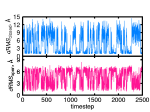
From the plot, we can observe multiple transitions between the open and the closed structures during the simulation.
3.2 Free energy profile (1D)
Here, we will calculate the Potential of Mean Force (PMF) along the dRMS, which we calculated in the previous section.
# Change directory
$ cd ../3.2_PMF_1D
$ ls
pmf_1d_drms.inp pmf_1d_edit.tcl pmf_1d_plot.gnu pmf_weight_2500_1.weight run.sh
We will use the GENESIS analysis tool pmf_analysis to calculate the PMF. Let’s take a look at the pmf_1d_drms.inp file:
[INPUT]
cvfile               = drms_{}.out # the CV file
weightfile           = pmf_weight_2500_{}.weight # weight file

[OUTPUT]
pmffile              = pmf_1d_drms.out

[OPTION]
nreplica             = 1
dimension            = 1
temperature          = 260
grids1               = 0 16 100 # (min max num_of_bins)
band_width1          = 0.1 # sigma of Gaussian kernel
is_periodic          = NO
The required input is the drms.out file and a weight file. When we use data from multiple simulations, we specify the weight of each data source at each frame. Here, we use only one trajectory, therefore the weight is simply 1 at each frame. Note that we named the weight file with a “1” suffix (pmf_weight_2500_1.weight). Under [OPTIONS] we specify the number of dimensions (1), the temperature of the simulation, and the desired bins. Since we specified that the number of required dimensions is 1, the PMF will be calculated with respect to the dRMS to the closed structure (column 2 in drms.out).
We will use the script run.sh which will add a suffix “1” to the name of the drms output file, run the GENESIS analysis tool pmf_analysis, and run the script pmf_1d_edit.tcl. The script pmf_1d_edit.tcl sets “Infinity” values to the maximal PMF value so that the data will be readable to the plotting script. After changing the GENESIS path in run.sh to your own path, let’s run the scripts:
# Run the PMF calculation and processing scripts
$ ./run.sh
# Plot the PMF
gnuplot pmf_1d_plot.gnu
(Note: pmf_analysis calculates the PMF in two different methods, here we use the first calculation method, please see the pmf_1d_drms.log log file for details).
We obtain the following PMF plot:
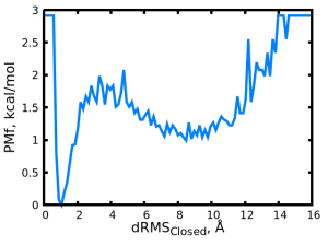 We can observe two minima, a deep and narrow basin at ~1 Å, representing the closed state, and another shallower basin at ~8 Å, representing the open state.
3.3 Free energy landscape (2D)
In the previous section, we calculated the PMF along the dRMS to the closed structure. Here, we will calculate the free energy landscape of the simulation along the two dRMS dimensions.
# Change directory
$ cd ../3.3_PMF
$ ls
pmf_2d_drms.inp pmf_2d_edit.tcl pmf_2d_plot.py pmf_weight_2500_1.weight run.sh
We will use the pmf_2d_drms.inp file, which is very similar to the pmf_1d_drms.inp file which we used for calculating the 1D PMF expect some minor changes:
[INPUT]
cvfile           = drms_{}.out  # the CV file
weightfile       = pmf_weight_2500_{}.weight  # weight file

[OUTPUT]
pmffile          = pmf_2d_drms.out

[OPTION]
nreplica         = 1
dimension        = 2
temperature      = 260
grids1           = 0 16 100 # (min max num_of_bins)
grids2           = 0 16 100 # (min max num_of_bins)
band_width1      = 0.1 # sigma of Gaussian kernel
band_width2      = 0.1 # sigma of Gaussian kernel
is_periodic1     = NO
is_periodic2     = NO
Under [OPTIONS] we specify that the number of dimensions is 2. Also, we specify an additional set of parameters for the 2nd dimension (e.g. “grids2”).
We will use the script run.sh which will add a suffix “1” to the name of the drms output file, run the GENESIS analysis tool pmf_analysis, and run the script pmf_edit.tcl. The script pmf_edit.tcl rewrites the output pmf file and writes grid information files, both are required for the plotting script pmf_plot.py . After changing the GENESIS path in run.sh to your own path, let’s run the scripts:
# Run the PMF calculation and processing scripts
$ ./run.sh
# Plot the PMF
./pmf_2d_plot.py
We obtain the 2D PMF along the dRMS CV:
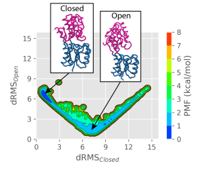
We can identify a stable closed basin (at low \( dRMS_{Closed} \)) values, and a shallower and wider open basin (at small \( dRMS_{Open} \) values). The reason for the open state being wider is that there are less contacts and therefore more fluctuations. We can confirm that snapshots from the simulations resemble the closed or the open states in the respective basins.
3.4 \( K_{eq} \)
We will now calculate the equilibrium coefficient \( K_{eq} \), defined as the ratio between the closed and the open populations during the simulation \( \left( K_{eq}=\frac{[closed]}{[open]} \right) \).
We will use the .tcl script keq_pmf.tcl which evaluate the populations in the Open and the Closed states according to the 1D PMF. The script requires the output file pmf_1d_drms_plot.out which was calculated in section 3.2.
# Change directory
$ cd ../3.4_Keq
# Run the script
$ tclsh keq_pmf.tcl ../3.2_PMF_1D/pmf_1d_drms_plot.out
Keq = 1.0666124327519946
The script outputs the \( K_{eq} \) value to the screen. The calculated value is close to 1, meaning that the simulation spends its time almost equally between the open and the closed states.
4. Estimating mixing parameters using MBAR analysis
The mixing parameters \( C \) and \( T_{mix} \) that we used in our simulation are unique to each system and were calibrated for this specific system so that the system will spend its time evenly between the open and the closed states while realizing frequent transitions between the states. Determination of proper parameters for DB mixing simulations is not trivial and usually requires multiple trial simulation rounds. Here, we show how to use the Multistate Bennet Acceptance Ratio (MBAR) analysis method [6] to estimate improved parameters without performing actual MD simulations. MBAR is a statistical method which estimates a physical quantity (for example the PMF) for an unsimulated condition by reweighing simulated data performed under various other conditions. The method is useful for cases in which multiple iterations of trial and error simulations are required for parameter tuning. We will now demonstrate how to use the method to estimate the PMF at some unsimulated condition (where a condition in this case is a set of mixing parameters \( C \) and \( T_{mix} \)) using existing simulation data.
# Change directory
$ cd ../../4_mbar
# Check the content of the "data" directory
$ ls data
drms1.out drms2.out drms3.out drms4.out run1.out run2.out run3.out run4.out
The “data” directory contains simulation .log files for four simulations (run1.out to run4.out) and corresponding dRMS files for those simulations (drms1.out to drms2.out). The simulation were performed under various conditions and their PMFs are shown in the following figure:
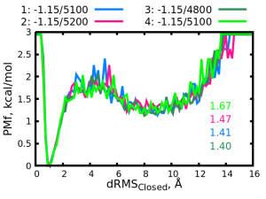
The mixing parameters \( C/T_{mix} \) are written in the legend and the \( K_{eq} \) values are written in the plot are in respective colors. The four simulations use similar parameters and the difference between them cannot be observed very well in the PMF plot but their \( K_{eq} \) values are different. We want to continue and find parameters which will give us \( K_{eq} \) closer to the target (~1). We could guess a set of parameters between those of simulations “1” and “2” from which \( K_{eq} \) are slightly over and under the target value, respectively. Normally, we would perform the next round of simulations with some guessed parameters, calculate the PMF and obtain its \( K_{eq} \). However, we can instead perform an MBAR calculation which will estimate the PMF at the guessed condition. The MBAR calculation is computationally much cheaper than an MD simulation, thus we can test multiple sets of parameters without using a large amount of computational resources and time.
During an MBAR calculation, a set of nonlinearly coupled equations are iteratively solved at the simulated conditions, which produces the weights of each of the simulated conditions with respect to the target condition. The MBAR calculation will be performed inside the the mbar directory:
# Change directory
$ cd mbar
# Check the content of the directory
$ ls
files_md_out.txt files_targets.txt mbar.inp mbar_permute.tcl mbar_target.tcl
The input file for the MBAR calculation is mbar.inp:
[INPUT]
cvfile             = run_permute_{}.out
targetfile         = run_target_{}.out

[OUTPUT]
weightfile         = run_weight_{}.weight
fenefile           = run_fene_{}.fene

[MBAR]
num_replicas       = 4                       # number of simulation data files
input_type         = MBGO                    # Multi-Basin GO simulation
temperature        = 260                     # temperature of simulation
target_temperature = 260                     # same as above in this case
dimension          = 1                       # dimension of CV
The input files run_permute_{}.out should contain the energies of each simulation, calculated for each of the simulated conditions. For example run_permute_1.out will contain the energies for simulation “1” calculated with the conditions (mixing parameters) of simulations “1”, “2”, “3”, and “4”. The input files run_target_{}.out should contain the energies of each simulation, calculated for the target (unsimulated) conditions. For example, run_target_1.out will contain the energies for simulation “1” calculated with the target conditions. We will use the .tcl scripts mbar_permute.tcl and mbar_target.tcl to create the run_permute_{}.out and run_target_{}.out files, respectively. Input files for two scripts are .out files from the simulations (run1.out to run4.out) as listed in the file files_md_out.txt. In addition, a file listing the target conditions, files_targets.txt is required for mbar_target.tcl:
$ cat files_targets.txt
5000 -1.0 0
The target conditions are listed in the order of \( T_{mix} \), \( C \), and the value of “0” which represents basinenergy2. The parameters listed in the file are for some unsimulated condition for which we want to estimate the PMF. Here, we only list one target condition so the file contains only one entry but multiple conditions can be estimated at once by listing them in the same file.
We will use the script run.sh to run mbar_permute.tcl, mbar_target.tcl, and mbar.inp:
# Run the script after changing the path to "bin" to you GENESIS installation path
$ ./run.sh
After the scripts have finished running, you should obtain run_permute_1.out to run_permute_4.out, run_target_1.out to run_target_4.out, run_weight_1.weight to run_weight_4.weight, and run_fene.fene.
Next, we will calculate the PMF for the target condition using the weight files from the MBAR calculation.
# Change directory
$ cd ../pmf
Let’s look at the pmf.inp file:
[INPUT]
cvfile             = ../data/drms{}.out
weightfile         = ../mbar/run_weight_{}.weight

[OUTPUT]
pmffile            = pmf.out

[OPTION]
nreplica           = 4
dimension          = 1
temperature        = 260
grids1             = 0 16 100
band_width1        = 0.1
is_periodic1       = NO
The file is very similar to the one we used in section 3.2. Here, we use four CV files (drms1.out to drms4.out of the simulated conditions), each with their respective weight file, and we set the number of replicas (nreplica) to 4.
The script run.sh calculates the PMF using pmf_analysis and calculate sss using keq_pmf.tcl. Let’s run the script:
# Run the calculation
$ ./run.sh
...
Keq = 1.227785582
We obtained the PMF and \( K_{eq} = 1.23 \). For comparison, we have performed an actual simulation with the target condition (\( T_{mix} = 5000, C = -1.0\)) and obtained \( K_{eq} = 1.05 \).
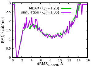
We see that MBAR mabaged to estimate a \( K_{eq} = 1.23 \) value which is close to the real (simulated) value. The accuracy of the MBAR estimation depends on several factors such as the amount of sampled data given as input and the the similarity of the input data to the target conditions. Here, we used a relatively small amount of input data (four input files) but still managed to obtain reasonable accuracy. Also, here we only performed one roiund of MBAR calculation, but we could continue and perform further rounds with a large variety of target parameters. Even better, we could simply input multiple target parameter sets in files_target.txt.
References
[1] Best et al., Structure 13.12 (2005): 1755-1763. [2] Daily et al., J. Mol. Biol. 400.3 (2010): 618-631. [3] Karanicolas and Brooks, Protein Sci. 11.10 (2002): 2351-2361. [4] Karanicolas and Brooks, J. Mol. Biol. 334.2 (2003): 309-325. [5] Domański et al., J. Phys. Chem. B 121.15 (2017): 3364-3375. [6] Shirts et al., J. Chem. Phys. 129.12 (2008): 124105.
Written by Ai Shinobu@RIKEN Laboratory for Biomolecular Function Simulation
April, 19, 2022