6.4 RNA in water
Contents
In this tutorial, we will perform a short simulation of a synthetic riboswitch called N1 [1]. It is a small RNA fragment, containing 27 nucleotides, able to bind aminoglycoside antibiotics and regulate the expression of genes located in the same mRNA. Its dynamics was thoroughly investigated using molecular dynamics simulations, both with and without various ligands [2,3]. For the simulations of the riboswitch, we are going to use Amber force field, which is considered to work well for the simulations of various RNA systems [2,3,4].
The tutorial files are available for download in this link: tutorial22-6.4. This tutorial consists of five steps: 1) system setup, 2) energy minimization, 3) equilibration, 4) production run, and 5) trajectory analysis. All control files for GENESIS are already included in the tutorial files.
# Download the tutorial file and confirm its content
$ cd /home/user/GENESIS/Tutorials
$ mv ~/Downloads/tutorial22-6.4.zip ./
$ unzip tutorial22-6.4.zip
$ cd tutorial22-6.4
$ ls
1_setup 2_minimize 3_equilibrate 4_production 5_analysis
1. Setup
The Amber force field contains the parameters for multiple water models, proteins, nucleic acids, lipids, glycans etc. All the information and appropriate references are available on the webpage of the Amber Project. Here, we are using the parameters for the TIP3P water model [5], monovalent ions [6] and ff99 force field for RNA [7] with the parmbsc0 [8] and χOL3 [9] corrections.
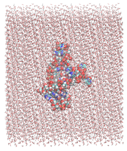
The pdb structure of the riboswitch with the ligand paromomycin can be downloaded from the RCSB Protein Data Bank (PDB ID 2mxs [1]). Since we are going to perform a simple simulation without any ligands, the paromomycin (PAR) residue should be removed. The PDB file without the ligand (2mxs_RNA-only.pdb) is already provided in the tutorial files in the “1_setup” directory. We are ready to use the Amber tleap program with the input file leap.inp to add water molecules and ions to the system to obtain the md.pdb file. The system is solvated with a 20 Å shell of TIP3P water molecules around the RNA molecule. 52 Na+ and 26 Cl− ions are added to neutralize the negative charge of the nucleic acid and achieve 100 mM NaCl concentration. At the same time, the Amber force field parameter file md.prm is generated. Detailed instructions and commands for working with tleap are provided in the tutorial 5.2. If you wish to skip this step, the output files md.pdb and md.prm are also included in the tutorial files.
# Change directory
$ cd 1_setup
$ ls
2mxs_RNA-only.pdb leap.inp md.pdb md.prm
# View the initial structure in VMD
$ vmd md.pdb -parm7 md.prm
If we look closely, we can see that there is a covalent bond between the hydrogens in the water molecules. This is because water molecules are treated as rigid in the SHAKE algorithm so the distance betweeen the hydrogens is kept fixed. There is no need to worry about this.
2. Minimization
The energy minimization will be performed using the steepest descent (SD) algorithm for 5000 time steps. At this stage, the positions of the non-hydrogen (heavy) atoms of the 27 residues of RNA are fixed by using positional restraints of 10 kcal/mol/Å2. The simulation is performed using periodic boundary conditions (PBC). The initial simulation box size is set according to the output log file from the tleap program. The particle mesh Ewald method (PME) is used for the long-range interactions. In contrast to the CHARMM force field, we do not use the switching distance for the van der Waals interactions, therefore the cutoff distance of 12.0 Å is set also for the switching distance value. Moreover, the dispersion correction “dispersion_corr = epress” is used for the simulations with the Amber force field. This parameter is set automatically, so we do not need to add it in the input file.
# Change directory
$ cd ../2_minimize
# View the contents of the control file
$ less INP
[INPUT]
prmtopfile      = ../1_setup/md.prm  # AMBER parameter topology file
pdbfile         = ../1_setup/md.pdb  # AMBER coordinate file
reffile         = ../1_setup/md.pdb  # reference PDB file for positional restraints

[OUTPUT]
dcdfile         = min.dcd  # DCD trajectory file
rstfile         = min.rst  # restart file

[ENERGY]
forcefield      = AMBER  # name of force field
electrostatic   = PME  # [CUTOFF/PME]
switchdist      = 12.0  # switch distance
cutoffdist      = 12.0  # cutoff distance
pairlistdist    = 13.5  # pair-list cutoff distance
pme_ngrid_x     = 80  # grid size_x in PME
pme_ngrid_y     = 80  # grid size_y in PME
pme_ngrid_z     = 72  # grid size_z in PME
water_model     = NONE  #

[MINIMIZE]
method          = SD    # minimization method
nsteps          = 5000   # number of minimization steps
eneout_period   = 5000   # energy output period
crdout_period   = 5000   # coordinates output period
rstout_period   = 5000   # restart output period
nbupdate_period = 10  # nonbonded output period

[BOUNDARY]
type            = PBC  #
box_size_x      = 79.661  # box size (x) in PBC
box_size_y      = 87.183  # box size (y) in PBC
box_size_z      = 73.748  # box size (z) in PBC

[SELECTION]
group1          = heavy and resno:1-27

[RESTRAINTS]
nfunctions      = 1  # number of functions
function1       = POSI  # restraint function type
constant1       = 10.0  # force constant
select_index1   = 1  # restraint group
Here, we will use 8 MPI processors (domain_x*domain_y*domain_z=2*2*2=8) and 1 OpenMP thread for the energy minimization using spdyn but the user can adjust these settings according to their computational resources’ architecture. After running the minimization, it is a good practice to visuallze the trajectory (by using a software such as VMD) and plot the potential energy, as shown in the previous tutorials.
Now, let’s run the minimization (the run should take ~5 minutes):
# Set the number of OpenMP threads
$ export OMP_NUM_THREADS=1

# Perform a simulation using spdyn by using 8 MPI processes
$ mpirun -np 8 /home/usr/GENESIS/bin/spdyn INP > log

# Visualize the trajectory in VMD
$ vmd ../1_setup/md.pdb -dcd min.dcd
3. Equilibration
Before the final production simulation we will perform equilibration. The equilibration will be performed in two steps, first in the canonical ensemble (NVT), and then in the isothermal-isobaric ensemble (NPT). The simulations will be performed at the target temperature 310.15 K, which is the temperature that was used for the experimental studies of the riboswitch. The directory for equilibration contains two control files:
# Change directory
$ cd ../3_equilibrate
$ ls
INP1 INP2
3.1 NVT-MD with positional restraints
The file INP1 will be used in the first equilibration step, which is carried out for 50 ps in the NVT ensemble. Note that the positional restraints applied to all non-hydrogen RNA atoms are now weaker so these atoms can move slightly more. The water molecules are not restrained thus they can move freely. The equations of motion are integrated using the velocity verlet integrator with the time step of 2 fs using the SHAKE algorithm [10] for the bonds involving hydrogen atoms. The Bussi thermostat is applied to control the temperature [11].
[INPUT]
prmtopfile      = ../1_setup/md.prm  # AMBER parameter topology file
pdbfile         = ../1_setup/md.pdb  # AMBER coordinate file
reffile         = ../1_setup/md.pdb  # reference PDB file for positional restraints
rstfile         = ../2_minimize/min.rst  # output file from minimization

[OUTPUT]
dcdfile         = eq1.dcd  # DCD trajectory file
rstfile         = eq1.rst  # restart file

[ENERGY]
forcefield      = AMBER  # name of force field
electrostatic   = PME  # [CUTOFF/PME]
switchdist      = 12.0  # switch distance
cutoffdist      = 12.0  # cutoff distance
pairlistdist    = 13.5  # pair-list cutoff distance
pme_ngrid_x     = 80  # grid size_x in PME
pme_ngrid_y     = 80  # grid size_y in PME
pme_ngrid_z     = 72  # grid size_z in PME

[BOUNDARY]
type            = PBC  #

[DYNAMICS]
integrator      = VVER  # type of integrator
nsteps          = 25000  # number of MD steps
timestep        = 0.002  # timestep of integration (ps)
eneout_period   = 5000  # energy output period
crdout_period   = 5000  # coordinates output period
rstout_period   = 25000  # restart output period
nbupdate_period = 10  # nonbonded output period

[CONSTRAINTS]
rigid_bond      = YES  # constraints all bonds involving hydrogen
fast_water      = YES  # use SETTLE algorithm
water_model     = WAT  #

[ENSEMBLE]
ensemble        = NVT  # NVE, NVT, NPT
tpcontrol       = BUSSI  # thermostat and barostat
temperature     = 310.15  # initial and target temperature (K)

[SELECTION]
group1          = heavy and resno:1-27

[RESTRAINTS]
nfunctions      = 1  # number of functions
function1       = POSI  # restraint function type
constant1       = 1.0  # force constant
select_index1   = 1  # restraint group
Let’s run the equilibration MD step1 (the run should take ~30 minutes):
# Set the number of OpenMP threads
$ export OMP_NUM_THREADS=4

# Perform a simulation using spdyn by using 8 MPI processes
$ mpirun -np 8 /home/usr/GENESIS/bin/spdyn INP1 > log1

# Visualize the trajectory in VMD
$ vmd ../1_setup/md.pdb -dcd eq1.dcd
3.2 NPT-MD with positional restraints
Next, we will perform the second step of equilibration (using INP2). There are two main differences between this step and the previous step. First, we switch the ensemble to NPT in order to regulate the box size. Second, we specify the target pressure P = 1 atm. The latter condition is a default setting for the simulations for the NPT ensemble, so we do not need to specify it in the input file. The Bussi barostat is applied to control the pressure [11]. All the parameters are printed in the output log file, so it is always possible to confirm them after the simulation.
[INPUT]
prmtopfile      = ../1_setup/md.prm  # AMBER parameter topology file
pdbfile         = ../1_setup/md.pdb  # AMBER coordinate file
reffile         = ../1_setup/md.pdb  # reference PDB file for positional restraints
rstfile         = ../eq1.rst  # output file from the previous step

[OUTPUT]
dcdfile         = eq2.dcd  # DCD trajectory file
rstfile         = eq2.rst  # restart file

[ENERGY]
forcefield      = AMBER  # name of force field
electrostatic   = PME  # [CUTOFF/PME]
switchdist      = 12.0  # switch distance
cutoffdist      = 12.0  # cutoff distance
pairlistdist    = 13.5  # pair-list cutoff distance
pme_ngrid_x     = 80  # grid size_x in PME
pme_ngrid_y     = 80  # grid size_y in PME
pme_ngrid_z     = 72  # grid size_z in PME

[BOUNDARY]
type            = PBC  #

[DYNAMICS]
integrator      = VVER  # type of integrator
nsteps          = 50000  # number of MD steps
timestep        = 0.002  # timestep of integration (ps)
eneout_period   = 5000  # energy output period
crdout_period   = 5000  # coordinates output period
rstout_period   = 50000  # restart output period
nbupdate_period = 10  # nonbonded output period

[CONSTRAINTS]
rigid_bond      = YES  # constraints all bonds involving hydrogen
fast_water      = YES  # use SETTLE algorithm
water_model     = WAT  #

[ENSEMBLE]
ensemble        = NPT  # NVE, NVT, NPT
tpcontrol       = BUSSI  # thermostat and barostat
temperature     = 310.15  # initial and target temperature (K)
pressure        = 1.0  # target pressure (atm)

[SELECTION]
group1          = heavy and resno:1-27

[RESTRAINTS]
nfunctions      = 1  # number of functions
function1       = POSI  # restraint function type
constant1       = 1.0  # force constant
select_index1   = 1  # restraint group
Let’s run the equilibration MD step2 (the run should take ~30 minutes):
# Set the number of OpenMP threads
$ export OMP_NUM_THREADS=4

# Perform a simulation using spdyn by using 8 MPI processes
$ mpirun -np 8 /home/usr/GENESIS/bin/spdyn INP2 > log2

# Visualize the trajectory in VMD
$ vmd ../1_setup/md.pdb -dcd eq2.dcd
It is also a good practice to observe the time course of the box size and pressure, as was demonstrated in previous tutorials.
4. Production
We will now perform a 400 ps production simulation in the isothermal-isobaric (NPT) ensemble without any restraints. Since it is safer to run the large production simulations in smaller parts, we will divide this simulation in two parts, using the input files INP1 and INP2.
# Change directory
$ cd ../4_production
$ ls
INP1 INP2
The contents of the INP1 file are shown below.
[INPUT]
prmtopfile      = ../1_setup/md.prm  # AMBER parameter topology file
pdbfile         = ../1_setup/md.pdb  # AMBER coordinate file
reffile         = ../1_setup/md.pdb  # reference PDB file for positional restraints
rstfile         = ../3_equilibrate/eq2.rst  # output file from the previous step

[OUTPUT]
dcdfile         = md1.dcd  # DCD trajectory file
rstfile         = md1.rst  # restart file

[ENERGY]
forcefield      = AMBER  # name of force field
electrostatic   = PME  # [CUTOFF/PME]
switchdist      = 12.0  # switch distance
cutoffdist      = 12.0  # cutoff distance
pairlistdist    = 13.5  # pair-list cutoff distance
pme_ngrid_x     = 80  # grid size_x in PME
pme_ngrid_y     = 80  # grid size_y in PME
pme_ngrid_z     = 72  # grid size_z in PME

[BOUNDARY]
type            = PBC  #

[DYNAMICS]
integrator      = VVER  # type of integrator
nsteps          = 100000  # number of MD steps
timestep        = 0.002  # timestep of integration (ps)
eneout_period   = 5000  # energy output period
crdout_period   = 5000  # coordinates output period
rstout_period   = 100000  # restart output period
nbupdate_period = 10  # nonbonded output period

[CONSTRAINTS]
rigid_bond      = YES  # constraints all bonds involving hydrogen
fast_water      = YES  # use SETTLE algorithm
water_model     = WAT  #

[ENSEMBLE]
ensemble        = NPT  # NVE, NVT, NPT
tpcontrol       = BUSSI  # thermostat and barostat
temperature     = 310.15  # initial and target temperature (K)
pressure        = 1.0  # target pressure (atm)
Let’s execute the two production runs (run INP2 after INP1 finishes ):
# Production run for 0-200 ps (restart from eq2.rst)
$ mpirun -np 8 /home/user/GENESIS/bin/spdyn INP1 > log1
# Production run for 200-400 ps (restart from md1.rst)
$ mpirun -np 8 /home/user/GENESIS/bin/spdyn INP2 > log2
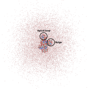
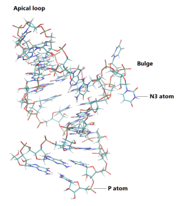
Since this simulation is run using periodic boundary conditions, water molecules can enter the neighboring “image” cells. It is possible to wrap the water molecules using VMD. You may have noticed in the production simulation that the RNA is very flexible, especially in the region of the apical loop and the bulge, which are the two regions in this RNA fragment that contain the bases not connected via the Watson-Crick hydrogen bonds. In the next section we will look closer at the RNA flexibility.:
# View the trajectory using VMD
$ vmd ../1_setup/md.pdb -dcd md2.dcd
vmd > pbc set {80 80 72} -all
vmd > pbc wrap -compound fragment -center origin -all
5. Analysis
The root-mean-square fluctuation (RMSF) is the fluctuation around an average position of the atoms or residues over a trajectory. It is a suitable measure when you want to compare the mobility of the residues of the structure, for example the movement of the RNA nucleotides which are connected with the Watson-Crick hydrogen bonds comaring to those that are not connected (here, they are in the apical loop and bulge regions). For this purpose, we will use the avecrd_analysis analysis tool, followed by the flccrd_analysis tool from the GENESIS analysis tool sets. The first tool calculates the average coordinates of the selected atoms, and the second tool calculates the RMSF. Input files for the analysis are provided. We will only use the second part of the production trajectory, as this part should be equilibrated better than the first part. The analysis will be performed for selected atoms in the bases of each nucleotide (namely, the atoms named N3). In this way, we can follow the dynamics of the bases only.
# Change directory
$ cd ../5_analysis
$ ls
INP1 INP2
# Perform analysis with the avecrd_analysis and flccrd_analysis tools
$ export OMP_NUM_THREADS=1
$ /home/user/GENESIS/bin/avecrd_analysis INP1 | tee run1.out
$ /home/user/GENESIS/bin/flccrd_analysis INP2 | tee run2.out
Several output files were produced during the calculation. The 4th column in the run2.rms file corresponds to the RMSF value in the units of Angstrom. It can be plotted with gnuplot for each of the 27 nucleotides:
# Plot the RMSF
$ gnuplot
gnuplot> set xlabel "Residue number"
gnuplot> set ylabel "RMSF [angstrom]"
gnuplot> plot "run2.rms" using 1:4 w lp
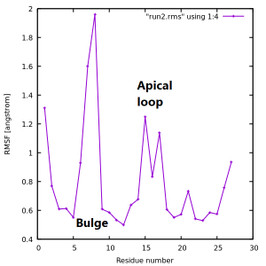
Can you plot the same RMSF graph for the phosphorus atoms (the atoms called P) in the RNA backbone? Do you notice any differences between those two graphs?
References
[1] Duchardt‐Ferner et al. Angew. Chem. Int. Ed. 49.35 (2010): 6216-6219. [2] Kulik et al. Nucleic Acids Res. 46.19 (2018): 9960-9970. [3] Chyży et al. Front. Mol. Biosci. 8 (2021): 12. [4] Sponer et al. Chem. Rev. 118.8 (2018): 4177-4338. [5] Jorgensen et al. J. Chem. Phys. 79.2 (1983): 926-935. [6] Joung and Cheatham J. Phys. Chem. B 112.30 (2008): 9020-9041. [7] Cornell et al. J. Am. Chem. Soc. 117.19 (1995): 5179-5197. [8] Pérez et al. Biophys. J. 92.11 (2007): 3817-3829. [9] Zgarbova et al. J. Chem. Theory Comput 7.9 (2011): 2886-2902. [10] Ryckaert et al. J. Comput. Phys. 23.3 (1977): 327-341. [11] Bussi et al. J. Chem. Phys. 126.1 (2007): 014101.
Written by Marta Kulik@RIKEN Theoretical molecular science laboratory & University of Warsaw