6.2 GPCR in a lipid bilayer
Contents
GPCR is one of the membrane proteins which regulate cell signaling between inside and outside of cells. In this tutorial, we learn how to setup the GPCR-membrane system by employing adenosine A2A receptor as an example.
1. Preparation
Let’s download the tutorial file (tutorial22-6.2). This tutorial consists of four steps: 1) system setup using CHARMM-GUI, 2) energy minimization and equilibration, 3) production run, and 4) trajectory analysis.
# Download the tutorial file$ unzip tutorial22-6.2.zip$ cd tutorial-6.2$ ls1_setup/ 2_min_equil/ 3_production/ 4_analysis/
2. Setup of initial structure using CHARMM-GUI
As described in tutorial 6.1, the setup of a bilayer system is difficult compared to solvation of globular proteins. If the system starts from a state far from equilibrium (for example, a random mixture of lipid and water molecules), it must take much time to equilibrate the system. The initial setup is considerably important to obtain the correct equilibrated state within short time. CHARMM-GUI provides a graphical user interface and many modules (Membrane builder etc.) which help us to build a protein-membrane system [1]. Here we demonstrate how to setup the initial structure of GPCR-membrane system using CHARMM-GUI.
Let’s go to top page of CHARMM-GUI. You need to login or register if you don’t have your account. From top page, please access “Input Generator” > “Membrane Builder” > “Bilayer Builder”. At the first step of the bilayer builder, we choose “Protein/Membrane System” and input a PDB id. From RCSB, we download “3pwh”, which is the thermostabilized adenosine A2A Receptor [2].
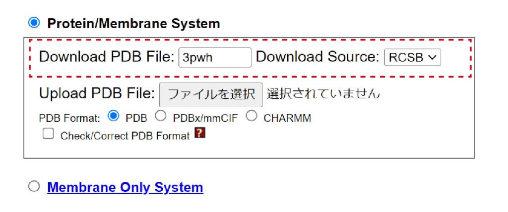
Figure 1. Choose “Protein/Membrane System” and input PDB id.
This PDB file contains not only GPCR but also a ligand. To include the ligand, check “Hetero” in “Model/Chain Selection Option”. The force field parameters for the ligand are automatically prepared using CGenFF. Segment id of the ligand is set to “HETA”.
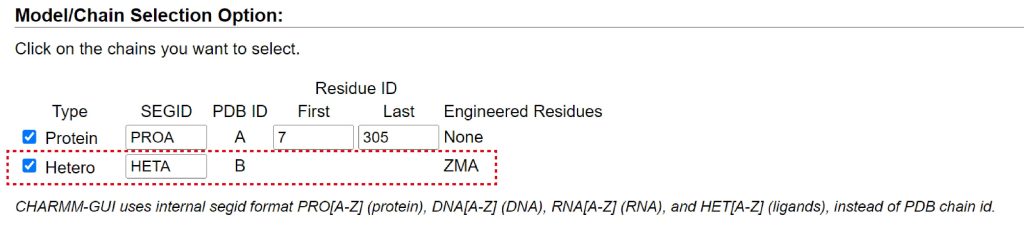
Figure 2. Check “Hetero” to include a ligand.
The orientation of the protein in membrane can be changed in “Orientation Options”. You should choose the adequate option for your system. In this tutorial, we choose “Align the First Principal Axis Along Z”.
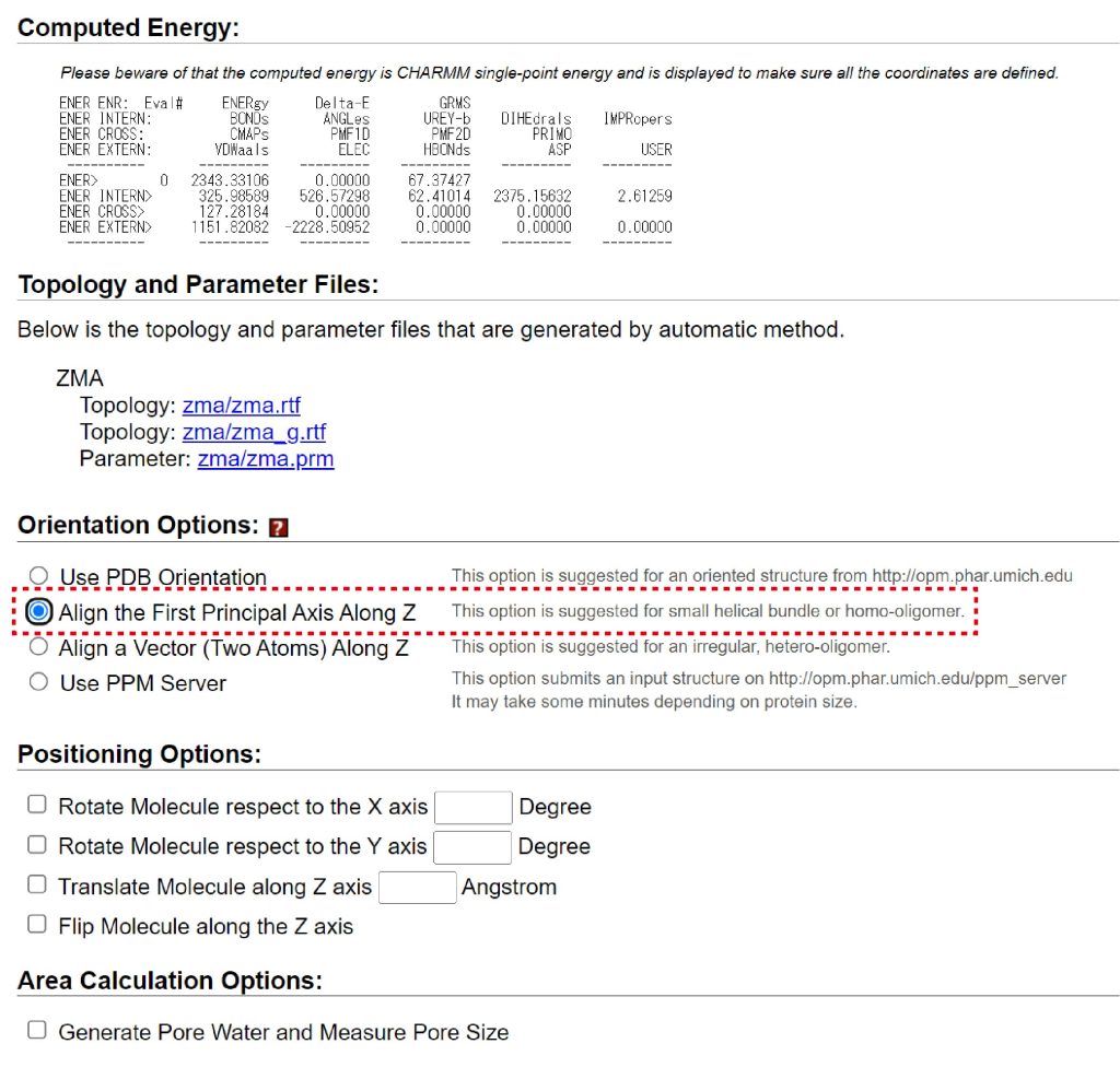
Figure 3. Check “Align the First Principal Axis Along Z” in “Orientation Options” to determine the orientation of GPCR in membrane.
In the next step, please make sure to view the structure in membrane from “view structure” (Figure 4). We obtain the orientation of GPCR in membrane shown in the left of Figure 5. If we check “Use PDB orientation” in “Orientation Options”, we obtain the wrong orientation shown in the right of Figure 5. GPCR is placed lateral to the membrane.
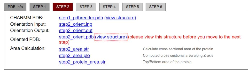
Figure 4. View the structure of GPCR in membrane.
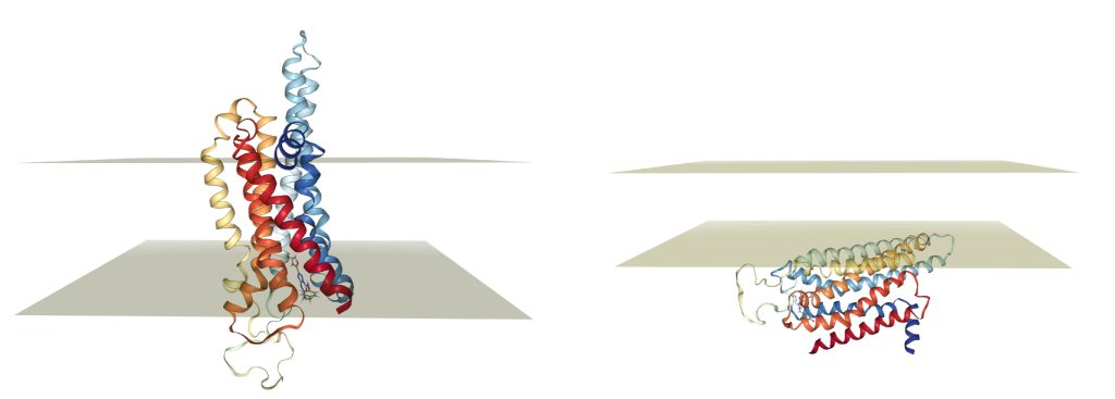
Figure 5. Orientations of GPCR in membrane. (Left) Orientation determined by “Align the First Principal Axis Along Z”. (Right) Orientation determined by “Use PDB Orientation”.
Next, we add “POPC” lipids and water molecules to the system. In tutorial 6.1, we determined the number of lipids and water molecules in the system by choosing “Number of lipid components”. Instead, here we choose “Ratios of lipid components” (Figure 6). We set “Length of X and Y” to 70 Å, and set “Upperleaflet Ratio” and “Lowerleaflet Ratio” of POPC to 1. After input the numbers, please click “Show the system info” to calculate the number of lipids. In our case, the numbers of POPC in the upper leaflet and lower leaflet are 56 and 55, respectively (Figure 7).
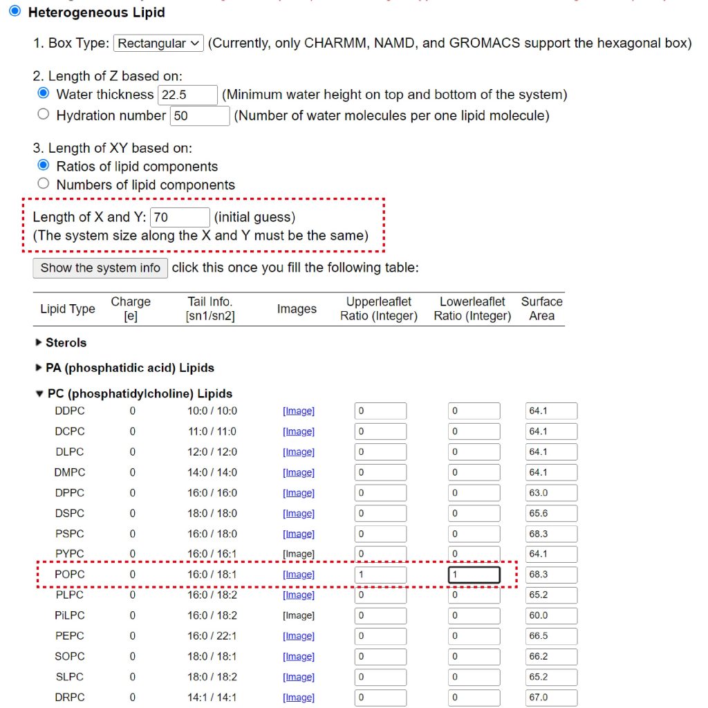
Figure 6. Addition of lipid to the system. Input lengths of X and Y and ratios of POPC in upper and lower leaflets.
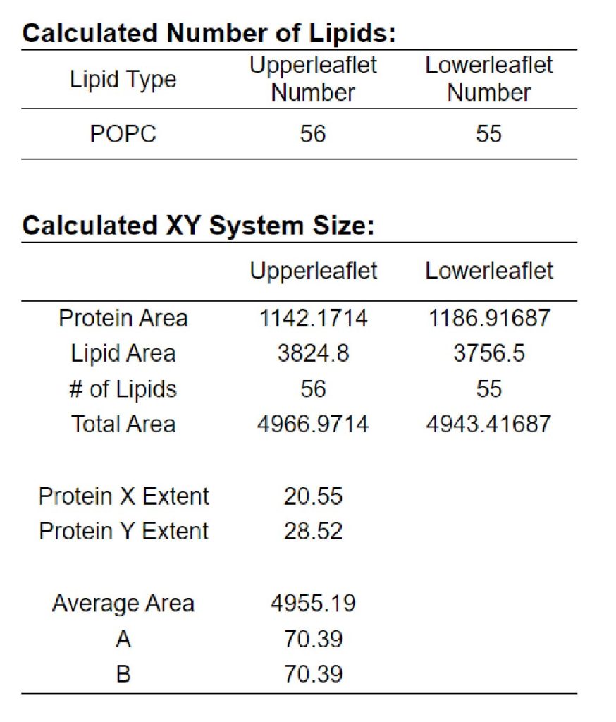
Figure 7. Number of lipid molecules added to the system.
The procedures after adding lipids are the same as in tutorial 6.1. We add salt to the system, check “GENESIS” in “Input Generation Options” and select the NPT ensemble in “Equilibration Options”, and download a set of the structure and parameter files for the GPCR-membrane system and input files for GENESIS by clicking “download.tgz” button.
After the download, let’s check the downloaded file.
# untar the downloaded tar file$ tar -xzvf charmm-gui.tgz$ lscharmm-gui-XXXXXXXXXXXX/$ cd charmm-gui-XXXXXXXXXXXX$ ls3pwh.cif findrings.py step2_orient.pdb step4.3_ion.out step5_assembly.psf3pwh_heta.crd genesis/ step2_protein_area.str step4.3_ion.pdb step5_assembly.str3pwh_heta.pdb glycan.yml step3_nlipids_lower.prm step4.3_ion.psf step5_input.inp3pwh_proa.crd input.config.dat step3_nlipids_upper.prm step4.3_ion.str step5_input.out3pwh_proa.fasta lipid_lib.tar.gz step3_packing.inp step4.3_ion_protmemb.crd step5_input_minimization.str3pwh_proa.model.pdb membrane_restraint.str step3_packing.out step4_components.str step6.1_equilibration.inp3pwh_proa.orig.map membrane_restraint2.str step3_packing.pdb step4_lipid.crd step6.2_equilibration.inp3pwh_proa.orig.pdb pentest.py step3_packing_head.crd step4_lipid.inp step6.3_equilibration.inp3pwh_proa.orig_init.in step1_pdbreader.crd step3_packing_head.pdb step4_lipid.out step6.4_equilibration.inp3pwh_proa.orig_init.out step1_pdbreader.inp step3_packing_head.psf step4_lipid.pdb step6.5_equilibration.inp3pwh_proa.orig_init.pdb step1_pdbreader.out step3_packing_pol.str step4_lipid.psf step6.6_equilibration.inp3pwh_proa.orig_init_init.fix step1_pdbreader.pdb step3_size.inp step4_lipid_lipid.crd step7_production.inp3pwh_proa.orig_opt.in step1_pdbreader.psf step3_size.out step4_lipid_lipid.psf toppar/3pwh_proa.orig_opt.log step1_pdbreader.str step3_size.str step4_lipid_pentest.out toppar.str3pwh_proa.orig_opt.pdb step2.2_ions_count.str step4.2_waterbox.crd step4_lipid_rings.str water_tmp.crd3pwh_proa.pdb step2_area.plo step4.2_waterbox.inp step5_assembly.crd zma/addCrystPdb.py* step2_area.str step4.2_waterbox.out step5_assembly.inpcheckfft.py step2_orient.crd step4.2_waterbox.psf step5_assembly.oldpsfcheckfft.str step2_orient.inp step4.3_ion.crd step5_assembly.outcrystal_image.str step2_orient.out step4.3_ion.inp step5_assembly.pdb$ cd genesis$ lsREADME step5_input.pdb step6.1_equilibration.inp step6.4_equilibration.inp step7_production.inprestraints/ step5_input.psf step6.2_equilibration.inp step6.5_equilibration.inp sysinfo.datstep5_input.crd step6.0_minimization.inp step6.3_equilibration.inp step6.6_equilibration.inp
The downloaded file contains several files used for setup of the system. “toppar” includes CHARMM force field file for proteins and solvent. “zma” includes CGenFF files for the ligand. “genesis” includes structure files (step5_input.pdb and step5_input.psf), control files for GENESIS (step*_***.inp), and files for local restraints (restraints/).
Let’s check the PDB file using PyMOL. Figure 8 shows the GPCR-POPC membrane system built by CHARMM-GUI.
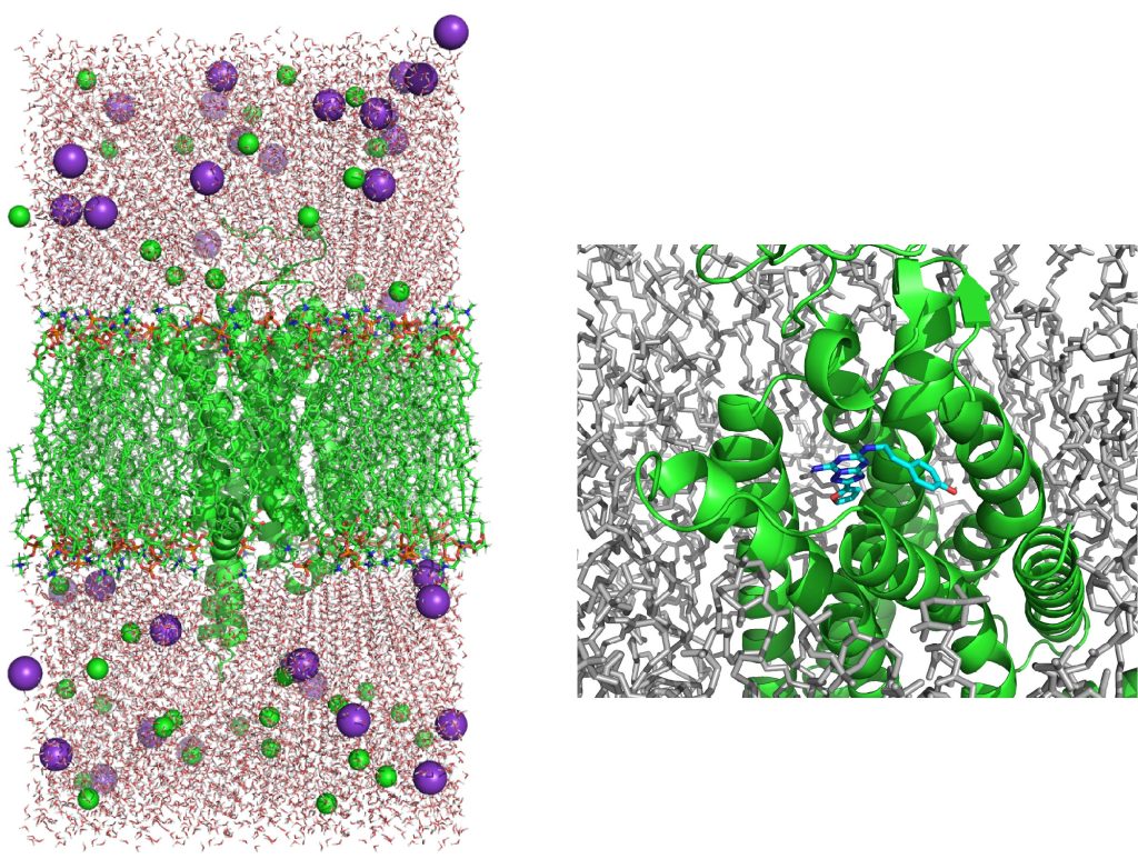
Figure 8. The membrane system of GPCR built by Membrane Builder in CHARMM-GUI. (Left) The side view of the system. (Right) The ligand bound to GPCR.
In this tutorial, we use only “toppar/”, “zma/”, “restraints/”, “step5_input.pdb” and “step5_input.psf” in the following sections. These files are included in “1_setup/” of tutorial22-6.2.zip, although “step5_input.pdb” and “step5_input.psf” are renamed “complex.pdb” and “complex.psf”, respectively.
# Check files in 1_setup/ of tutorial-6.2$ cd 1_setup$ lscomplex.pdb complex.psf restraints/ toppar/ zma/
3. Minimization and equilibration
3. 1. Perform MD simulations using spdyn
Let’s move to “2_min_equil” and check control files for GENESIS.
$ cd ../2_min_equil/$ lsrun_eq1.inp run_eq2.inp run_eq3.inp run_eq4.inp run_eq5.inp run_eq6.inp run_eq7.inp run_min.inp
Structure and force field files generated by CHARMM-GUI are set to each control file at [INPUT] section.
[INPUT]topfile = ../1_setup/toppar/top_all36_prot.rtf, …parfile = ../1_setup/toppar/par_all36m_prot.prm, …strfile = ../1_setup/toppar/toppar_all36_moreions.str, …psffile = ../1_setup/complex.psf # protein structure filepdbfile = ../1_setup/complex.pdb # PDB filereffile = ../1_setup/complex.pdb # Reference PDB filelocalresfile = ../1_setup/restraints/run_min.dihe # local restraint file
The procedures of minimization and equilibration are almost the same as tutorial 6.1, but there are some differences because our system includes not only lipid but also the GPCR and its ligand. In addition to local restraints and positional restraints for lipid molecules in tutorial 6.1, we also apply positional restraints to the protein and ligand during minimization and equilibration. The setting of each step is summarized in the following table:
| Step | Ensemble | Integrator | Step | Δt (fs) | k [local] | k [Pz] | k [bb] | k [sc] |
| 0 | Min | – | 5,000 | – | 250 | 2.5 | 10 | 5 |
| 1 | NVT | VVER | 25,000 | 1 | 250 | 2.5 | 10 | 5 |
| 2 | NVT | VVER | 25,000 | 1 | 100 | 2.5 | 5 | 2.5 |
| 3 | NPT | VVER | 25,000 | 1 | 50 | 1 | 2.5 | 1 |
| 4 | NPT | VVER | 50,000 | 2 | 50 | 0.5 | 1 | 0.5 |
| 5 | NPT | VVER | 50,000 | 2 | 25 | 0.1 | 0.5 | 0.1 |
| 6 | NPT | VVER | 100,000 | 2 | 0 | 0 | 0.1 | 0 |
| 7 | NPT | VRES | 400,000 | 2.5 | 0 | 0 | 0 | 0 |
k [local], k [Pz], k [bb], and k [sc] represent the force constants for local restraints of lipid’s dihedrals, positional restraints of phosphate atoms, positional restraints of the backbone atoms of the protein and the heavy atoms of the ligand, and positional restraints of the side-chain atoms of the protein, respectively. The positional restraints of phosphate atoms are set along the Z axis of the system. As the equilibration progresses, all restraints are slowly reduced and the timestep is gradually increased. In Step 7, the r-RESPA integrator (VRES) is used for final equilibration. VRES requires “group_tp = yes” in the [ENSEMBLE] section if GENESIS 2.0 is used. The simulation with NPT is carried out with the semi-iso option, which keeps the ratio of the box size in the x and y directions. The above equilibration protocol is based on Ref.[1], although the NPT ensemble is used instead of NPAT.
Let’s execute GENESIS spdyn by following commands.
# Set path to the bin directory of GENESIS
# This depdends on your system.$ GENESIS_BIN_DIR=...
$ export spdyn=$GENESIS_BIN_DIR/spdyn# To perform MD simulations, we use 8 MPI processes and 4 threads for each MPI process.# For these calculations, at least 8 * 4 = 32 CPU cores are required.# Please change these values for your computational environment.$ export OMP_NUM_THREADS=4# 5000 step energy minimization# with dihedral angle restraint (k = 250 kcal/mol)# z-positional restraint on P atoms (k = 2.5 kcal/mol/Angs^2)# positional restraint on backbone atoms of GPCR and heavy atoms of the ligand (k = 10 kcal/mol/Angs^2)# positional restraint on side-chain atoms of GPCR (k = 5 kcal/mol/Angs^2)$ mpirun -n 8 $spdyn run_min.inp > run_min.out# 25 ps MD in the NVT ensemble# with dihedral angle restraint (k = 250 kcal/mol)# z-positional restraint on P atoms (k = 2.5 kcal/mol/Angs^2)# positional restraint on backbone atoms of GPCR and heavy atoms of the ligand (k = 10 kcal/mol/Angs^2)# positional restraint on side-chain atoms of GPCR (k = 5 kcal/mol/Angs^2)$ mpirun -n 8 $spdyn run_eq1.inp > run_eq1.out# 25 ps MD in the NVT ensemble# with dihedral angle restraint (k = 100 kcal/mol)# z-positional restraint on P atoms (k = 2.5 kcal/mol/Angs^2)# positional restraint on backbone atoms of GPCR and heavy atoms of the ligand (k = 5 kcal/mol/Angs^2)# positional restraint on side-chain atoms of GPCR (k = 2.5 kcal/mol/Angs^2)$ mpirun -n 8 $spdyn run_eq2.inp > run_eq2.out# 25 ps MD in the NPT ensemble# with dihedral angle restraint (k = 50 kcal/mol)# z-positional restraint on P atoms (k = 1 kcal/mol/Angs^2)# positional restraint on backbone atoms of GPCR and heavy atoms of the ligand (k = 2.5 kcal/mol/Angs^2)# positional restraint on side-chain atoms of GPCR (k = 1 kcal/mol/Angs^2)$ mpirun -n 8 $spdyn run_eq3.inp > run_eq3.out# 100 ps MD in the NPT ensemble# with dihedral angle restraint (k = 50 kcal/mol)# z-positional restraint on P atoms (k = 0.5 kcal/mol/Angs^2)# positional restraint on backbone atoms of GPCR and heavy atoms of the ligand (k = 1 kcal/mol/Angs^2)# positional restraint on side-chain atoms of GPCR (k = 0.5 kcal/mol/Angs^2)$ mpirun -n 8 $spdyn run_eq4.inp > run_eq4.out# 100 ps MD in the NPT ensemble# with dihedral angle restraint (k = 25 kcal/mol)# z-positional restraint on P atoms (k = 0.1 kcal/mol/Angs^2)# positional restraint on backbone atoms of GPCR and heavy atoms of the ligand (k = 0.5 kcal/mol/Angs^2)# positional restraint on side-chain atoms of GPCR (k = 0.1 kcal/mol/Angs^2)$ mpirun -n 8 $spdyn run_eq5.inp > run_eq5.out# 200 ps MD in the NPT ensemble# with positional restraint on backbone atoms of GPCR and heavy atoms of the ligand (k = 0.1 kcal/mol/Angs^2)$ mpirun -n 8 $spdyn run_eq6.inp > run_eq6.out#1 ns MD in the NPT ensemble without any restraints using VRES with 2.5-fs time step$ mpirun -n 8 $spdyn run_eq7.inp > run_eq7.out
3. 2. Check the structures and physical properties
After the equilibration steps, check the structures of the whole system by using visualization software (PyMOL, VMD, etc.).
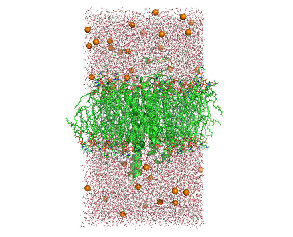
Figure 9. The system after the equilibration.
Also, check the physical properties: energies, temperatures, and volume of the system. First, extract the “INFO” lines from output files to individual files.
$ grep INFO run_min.out > log_min.dat$ for i in {1..7}; dogrep INFO run_eq${i}.out > log${i}.datdone
Start up gnuplot. Plot the energy changes in minimization by inputting the following command on gnuplot.
set xlabel "Step"set ylabel "Energy (kcal/mol)"p "log_min.dat" u 2:3 w l ti "min"
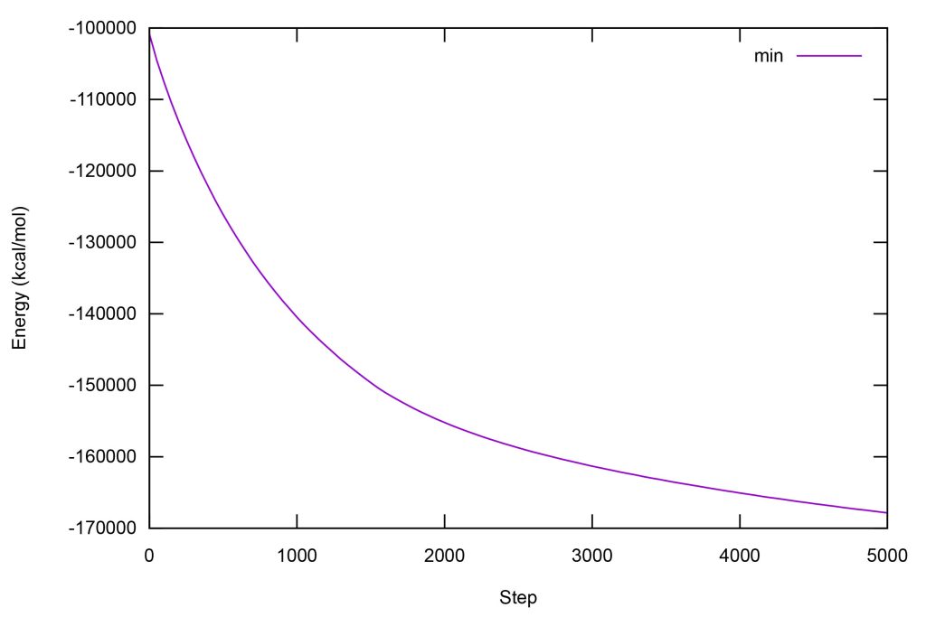
Figure 10. Changes in the total potential energy during minimization.
Plot temperatures of the system by inputting the following command on gnuplot.
set xlabel "Time (ps)"set ylabel "Temperature (K)"p [][280:325] \"log1.dat" u 3:17 w l ti "eq1", \"log2.dat" u (\$3+25):17 w l ti "eq2", \"log3.dat" u (\$3+50):17 w l ti "eq3", \"log4.dat" u (\$3+75):17 w l ti "eq4", \"log5.dat" u (\$3+175):17 w l ti "eq5", \"log6.dat" u (\$3+275):17 w l ti "eq6", \"log7.dat" u (\$3+475):16 w l ti "eq7"
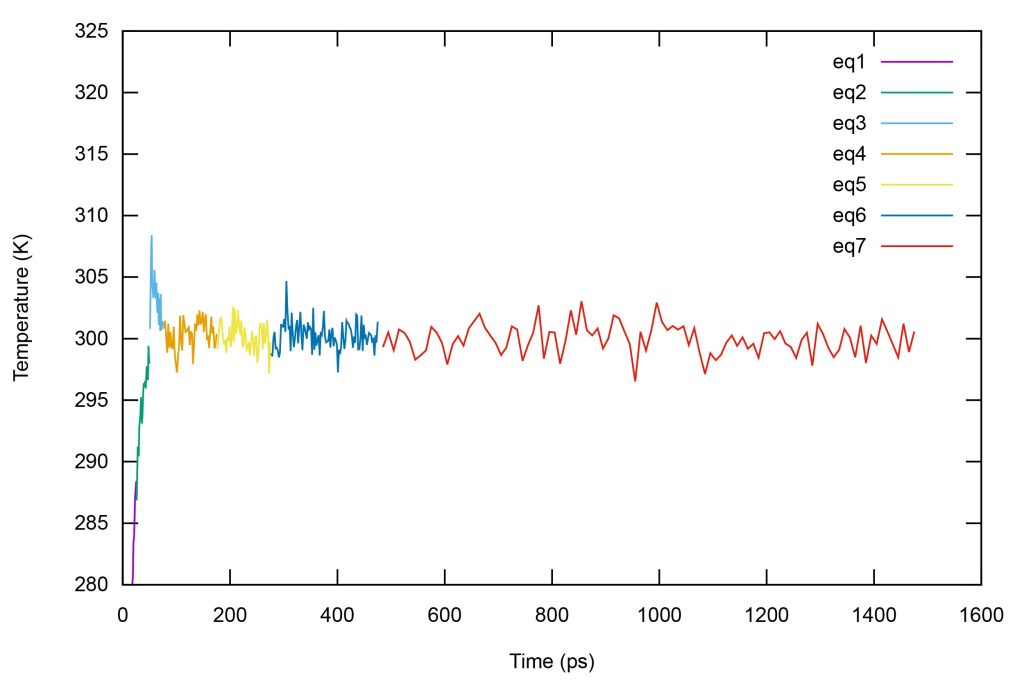
Figure 11. Time series of temperatures of the system during equilibration.
Plot the box size in the x direction by inputting the following command on gnuplot.
set xlabel "Time (ps)"set ylabel "Box x size (angstrom)"p [][66:72] \"log3.dat" u (\$3+50):19 w l ti "eq3", \"log4.dat" u (\$3+75):19 w l ti "eq4", \"log5.dat" u (\$3+175):19 w l ti "eq5", \"log6.dat" u (\$3+275):19 w l ti "eq6", \"log7.dat" u (\$3+475):18 w l ti "eq7"
For z direction.
set xlabel "Time (ps)"set ylabel "Box z size (angstrom)"p [][117:132] \"log3.dat" u (\$3+50):21 w l ti "eq3", \"log4.dat" u (\$3+75):21 w l ti "eq4", \"log5.dat" u (\$3+175):21 w l ti "eq5", \"log6.dat" u (\$3+275):21 w l ti "eq6", \"log7.dat" u (\$3+475):20 w l ti "eq7"
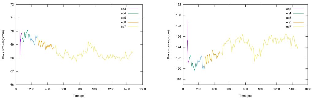
Figure 12. Time series of the box size during equilibration. (Left) x direction. (Right) z direction.
If there is no problem, we move on to the production.
3. 3. Note on equilibration
In above equilibration processes, NVT equilibration times are very short (25 ps). However, never increase the time steps for NVT equilibration. When the NVT equilibration time is increased to 1 ns, a large bubble appears in the system (Figure 13). The volume of the system in the initial state built by CHARMM-GUI might be too large for the number of molecules in the system or the temperature of 300 K. The bubble does not disappear even in NPT equilibration and breaks the lipid bilayer (Figure 14). Even if the simulation time in NPT is increased, the system never recover the correct equilibration state. You had better rapidly go through NVT processes before bubbles appear in your system.
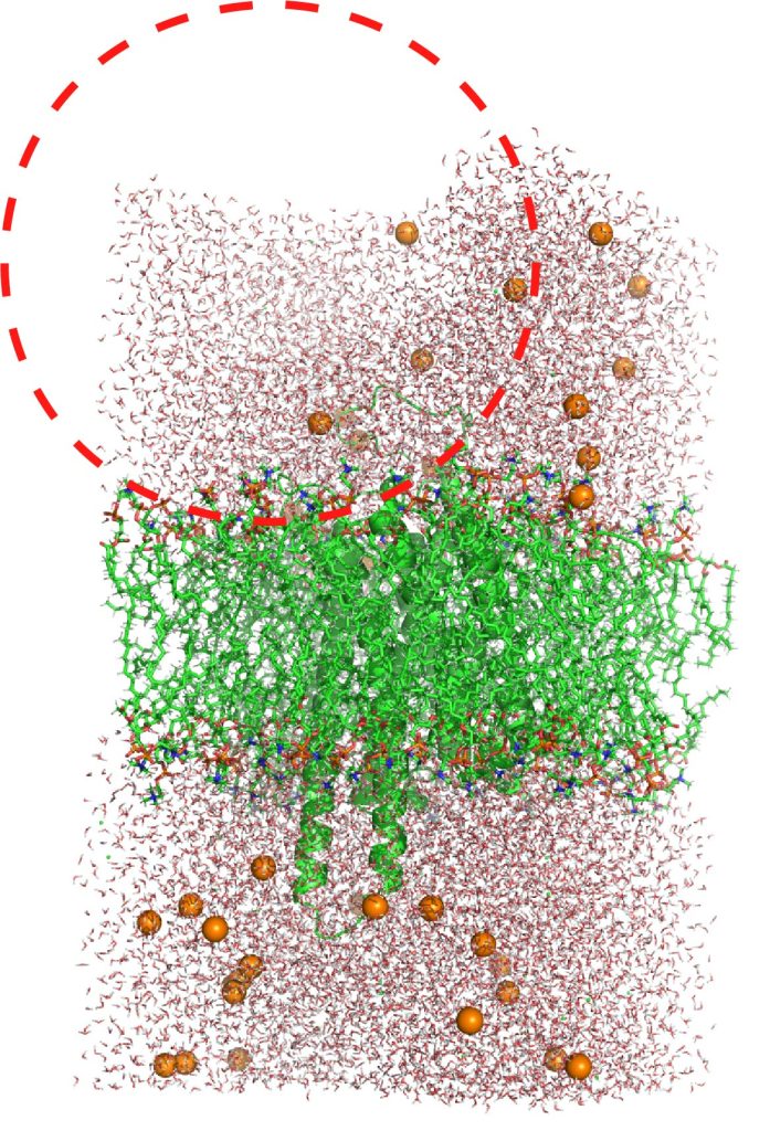
Figure 13. A bubble in the system. The dashed red line indicates a large void space.
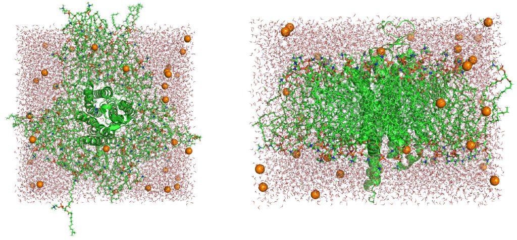
Figure 14. Collapse of the membrane system. (Left) The top view of the system. (Right) The side view of the system.
4. Production
Let’s perform production run. Move to “3_production” and check control files for GENESIS.
$ cd ../3_production/$ lsrun_prod.inp
In this tutorial, we perform the 10-ns MD simulation with NPT ensemble using r-RESPA integrator with 2.5-fs time step. Execute the following commands.
# Set path to the bin directory of GENESIS$ export spdyn=$GENESIS_BIN_DIR/spdyn# To perform MD simulations, we use 8 MPI processes and 4 threads for each MPI process.# For these calculations, at least 8 * 4 = 32 CPU cores are required.# Please change these values for your computational environment.$ export OMP_NUM_THREADS=4# 10 ns MD with NPT ensemble using VRES$ mpirun -n 8 $spdyn run_prod.inp > run_prod.out
Check the trajectory obtained by the production run using VMD. As shown in the below movie, the system is stable during the production run.
5. Analysis
Let’s analyze the resulting trajectory. Move to the “4_analysis” directory.
$ cd ../4_analysis$ lsrmsd/ rmsf/
Here we calculate the root-mean-square displacement (RMSD) and root-mean-square fluctuation (RMSF) of GPCR.
5. 1. RMSD of GPCR
Move to the “rmsd” directory.
$ cd rmsd$ lsrmsd.inprun.sh
The RMSD can be calculated using rmsd_analysis in GENESIS analysis tools. rmsd.inp is the input file for calculation of the RMSD of heavy atoms of GPCR.
[INPUT]psffile = ../../1_setup/complex.psfreffile = ../../1_setup/complex.pdb[OUTPUT]rmsfile = rmsd.dat # RMSD file[TRAJECTORY]trjfile1 = ../../3_production/run_prod.dcd # trajectory filemd_step1 = 1000 # number of MD stepsmdout_period1 = 1 # MD output periodana_period1 = 1 # analysis periodrepeat1 = 1trj_format = DCD # (PDB/DCD)trj_type = COOR+BOX # (COOR/COOR+BOX)trj_natom = 0 # (0:uses reference PDB atom count)[SELECTION]group1 = heavy and segid:PROA[FITTING]fitting_method = TR+ROT # NO/TR+ROT/TR/TR+ZROT/XYTR/XYTR+ZROTfitting_atom = 1 # atom groupzrot_ngrid = 10 # number of z-rot gridszrot_grid_size = 1.0 # z-rot grid sizemass_weight = NO # mass-weight is not applied[OPTION]check_only = NO # only checking input files (YES/NO)allow_backup = NO # backup existing output files (YES/NO)analysis_atom = 1 # atom group
run.sh is the script file for executing rmsd_analysis.
#!/bin/bash
rm rmsd.dat$GENESIS_BIN_DIR/rmsd_analysis ./rmsd.inp > rmsd.log
Execute run.sh and plot rmsd.dat using gnuplot.
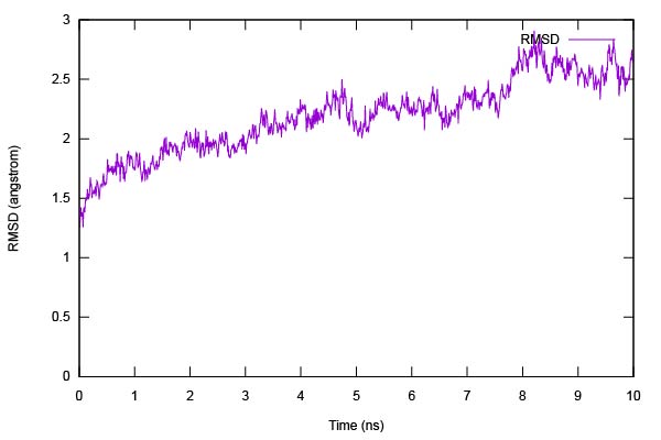
Figure 15. Time series of the RMSD of heavy atoms of GPCR.
5. 2. RMSF of GPCR
Move to the “rmsf” directory.
$ cd ../rmsf$ lsavecrd.inpflccrd.inprun.sh
First, calculate the average structure from the obtained trajectory using avecrd_analysis in GENESIS analysis tools. avecrd.inp is the input file for calculation of the averaged structure.
[INPUT]reffile = ../../1_setup/complex.pdb # PDB file[OUTPUT]pdbfile = run1.pdb # PDB filermsfile = run1.rms # RMSD filepdb_avefile = run1_ave.pdb # PDB file (Averaged coordinates of analysis atoms)pdb_aftfile = run1_aft.pdb # PDB file (Averaged coordinates of fitting atoms)[TRAJECTORY]trjfile1 = ../../3_production/run_prod.dcdmd_step1 = 1000mdout_period1 = 1ana_period1 = 1repeat1 = 1trj_format = DCD # (PDB/DCD)trj_type = COOR # (COOR/COOR+BOX)trj_natom = 0 # (0:uses reference PDB atom count)[SELECTION]group1 = an:CA and segid:PROA[FITTING]fitting_method = TR+ROT # methodfitting_atom = 1 # atom groupmass_weight = YES # mass-weight is applied[OPTION]check_only = NO # (YES/NO)num_iterations = 10 # number of iterationsanalysis_atom = 1 # analysis target atom group
Then, calculate the RMSF of C_alpha atoms from the averaged structure using flccrd_analysis in GENESIS analysis tools. flccrd.inp is the input file for calculation of the RMSF of GPCR.
[INPUT]reffile = ../../1_setup/complex.pdb # PDB filepdb_avefile = run1_ave.pdb # PDB file (Average coordinates)pdb_aftfile = run1_aft.pdb # PDB file (Fitted Average coordinates)[OUTPUT]pcafile = run2.pca # PCA filermsfile = run2.rms # RMSF and B-factor filevcvfile = run2.vcv # Variance-Covarience Matrix filecrsfile = run2.crs # CRS file[TRAJECTORY]trjfile1 = ../../3_production/run_prod.dcdmd_step1 = 1000mdout_period1 = 1ana_period1 = 1repeat1 = 1trj_format = DCD # (PDB/DCD)trj_type = COOR # (COOR/COOR+BOX)trj_natom = 0 # (0:uses reference PDB atom count)[SELECTION]group1 = an:CA and segid:PROA[FITTING]fitting_method = TR+ROT # methodfitting_atom = 1 # atom groupmass_weight = YES # mass-weight is applied[OPTION]check_only = NO # (YES/NO)analysis_atom = 1 # analysis target atom group
run.sh is the script file for executing avecrd_analysis and flccrd_analysis.
#!/bin/bash
rm run1* run2*$GENESIS_BIN_DIR/avecrd_analysis ./avecrd.inp > avecrd.out$GENESIS_BIN_DIR/flccrd_analysis ./flccrd.inp > flccrd.out
Let’s execute run.sh and plot rmsd.dat using gnuplot.
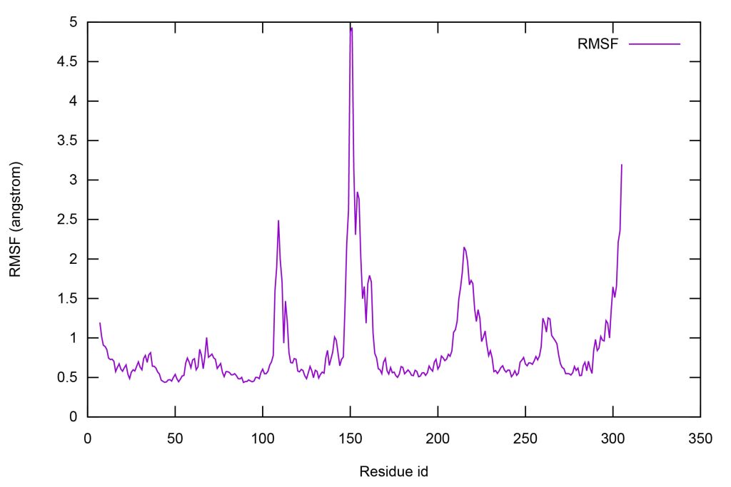
Figure 16. The RMSF of each residue of GPCR.
From Figure 16, the residues around 150 largely fluctuate compared to other residues. These residues are loop on the outside of membrane.
6. References
- S. Jo, T. Kim,W. Im, Automated Builder and Database of Protein/Membrane Complexes for Molecular Dynamics Simulations, PLoS ONE, 2, e880 (2007).
- A. S. Doré, N. Robertson, J. C. Errey, I. Ng, K. Hollenstein, B. Tehan, E. Hurrell, K. Bennett, M. Congreve, F. Magnani, C. G. Tate, M. Weir, F. H. Marshall, Structure of the Adenosine A2A Receptor in Complex with ZM241385 and the Xanthines XAC and Caffeine, Structure 19, 1283-1293 (2011).
Written by Hiraku Oshima@RIKEN BDR
February 18, 2022