4.3 Statistical analysis of the trajectory data by Python
Contents
Note: this tutorial is a simple introduction to using python (version 3.x) and packages such as NumPy and matplotlib to do some fundamental statistical analysis of simulation results. If you want to use python to parse MD trajectories, please try specific libraries such as MDTraj and MDAnalysis, which are beyond the scope of the current tutorial. Please refer to the website of python for a basic programming guide and get help from PyPI or anaconda about how to install packages.
Preparation
Please download the files for tutorial-4.3.
# Download the tutorial file
$ cd ~/GENESIS_Tutorials-2022/Works
$ mv ~/Downloads/tutorial22-4.3.zip ./
$ unzip tutorial22-4.3.zip

# Let's clean up the directory
$ mv tutorial22-4.1.zip ./TRASH

# Let's take a note
$ echo "tutorial-4.3: Trajectory analysis using python" >> README

$ cd ./tutorial-4.3
$ ls
Analysis1 Analysis2.1 Analysis2.2
1. Basic statistics
We first learn to do some basic statistical analysis, such as calculating the average and standard deviation and finding out the maximum/minimum values. These tasks can be easily accomplished by writing python scripts. In the following examples, we will analyze the energy data obtained in Tutorial 3.1.
# Change directory for statistics analysis
$ cd Analysis1
$ ls
energy.log 01_list.py 02_numpy.py
1.1 Using the “list” data structure
In this part, we show how to use the basic list structure to store data read from a file and how to compute the average and standard deviation.
We use the script 01_list.py to do everything. You can take a look at the file by running cat 01_list.py:
#!/usr/bin/env python3

# analyze the 5th column
i_col = 5

# use the list ene_data to store energy values
ene_data = []
with open("./energy.log", "r") as ene_file:
    for line in ene_file:
        ene_value = float(line.split()[i_col - 1])
        ene_data.append(ene_value)

# print length of the list
len_ene_data = len(ene_data)
print("Length of the energy list:", len_ene_data)

# find out the max/min
print("Maximum of column {0:>2d}: {1:>12.4f}".format(i_col, max(ene_data)))
print("Minimum of column {0:>2d}: {1:>12.4f}".format(i_col, min(ene_data)))

# calculate the average
ene_ave = sum(ene_data) / len_ene_data
print("Average of column {0:>2d}: {1:>12.4f}".format(i_col, ene_ave))

# calculate the standard deviation
ene_std = (sum((e - ene_ave)**2 for e in ene_data) / len_ene_data)**0.5
print("Standard deviation of column {0:>2d}: {1:>12.4f}".format(i_col, ene_std))
i_colis an integer variable to specify the column of interest.ene_datais the list we use to store energy data.- all the data is read from
"./energy.log"within theforloop:lineis a “string” variable to store every line in the file;line.split()simply splits the line into a list of words;float()is a function to convert a “string” into a “float”;append()is a function to add new values to the end of theene_datalist.
len()is a function used to get the length of a list.max()andmin()are the functions used to find out the maximum and minimum values from the list, respectively.sum()is a function used to calculate the sum of a list.- in the calculation of the standard deviation, we use a python tactic called “list comprehension” to quickly construct a new list:
(e - ene_ave)**2 for e in ene_data, whose elements are the squared deviations from the average. format()inserts the values saved in a variable to the message to be printed out.
Now let’s execute the script:
$ ./01_list.py         # or: python3 01_list.py
Length of the energy list: 1000
Maximum of column 5: 7.3745
Minimum of column 5: -10.2807
Average of column 5: -1.5140
Standard deviation of column 5: 2.8306
1.2 Using the “numpy.ndarray” data structure
In this part, we show an alternative way to get the maximum/minimum, average, and standard deviation values using the numpy library. numpy is a Python “package” or “module” that provides a multidimensional array object and various functions for fast operations on arrays.
The program is in the 02_numpy.py file:
#!/usr/bin/env python3

import numpy as np

# analyze the 5th column
i_col = 5

# use array ene_data to store energy values
ene_data = np.loadtxt("./energy.log", usecols=i_col - 1)

# print length of the list
len_ene_data = ene_data.size
print("Length of the energy list:", len_ene_data)

# find out the max/min
print("Maximum of column {0:>2d}: {1:>12.4f}".format(i_col, ene_data.max()))
print("Minimum of column {0:>2d}: {1:>12.4f}".format(i_col, ene_data.min()))

# calculate the average
ene_ave = ene_data.mean()
print("Average of column {0:>2d}: {1:>12.4f}".format(i_col, ene_ave))

# calculate the standard deviation
ene_std = ene_data.std()
print("Standard deviation of column {0:>2d}: {1:>12.4f}".format(i_col, ene_std))
Compared with 01_list.py, this new script looks much simpler. Actually, in many cases, numpy can simplify the development of programs. We list out the main differences between the two versions in the following:
import numpy as npis used to declare the usage ofnumpy.np.loadtxt()is a function used to read formatted data from file; the return value is an array (“ene_data“).sizeof an array is the number of elements (be aware thatsizeis not a function).max()andmin()are now used as member functions of the arrayene_data.mean()calculates the average of an array.std()directly computes the standard deviation.
Let’s run this new script:
$ ./02_numpy.py         # or: python3 02_numpy.py
Length of the energy list: 1000
Maximum of column 5: 7.3745
Minimum of column 5: -10.2807
Average of column 5: -1.5140
Standard deviation of column 5: 2.8306
As can be seen, the results are the same as the ones we computed with the 01_list.py.
2. Histogram analysis
A histogram is an approximate representation of the distribution of numerical data. In section 2, we are going to compute and plot one-dimensional (1D) and two-dimensional (2D) histograms from the MD simulation results.
2.1 1D-Histogram
First, we analyze the distance data (output.dis) obtained from Tutorial 3.2 and plot a 1D histogram. There are different ways to get a histogram. For example, the data visualization package matplotlib provides a matplotlib.pyplot.hist function, which directly draws a histogram. Alternatively, numpy also has a function numpy.histogram. We can first use this function to get the result and then use matplotlib to plot it. Of course, we can also use the list data structure to construct a histogram by “manually” counting the number of data in each predefined bin. Here we show the simplest way with the matplotlib.pyplot.hist function.
# Change directory to 1d-histogram analysis
$ cd ../Analysis2.1
$ ls
hist1d.py output.dis
The program is in the file hist1d.py:
#!/usr/bin/env python3

import numpy as np
import matplotlib.pyplot as plt

# load data from file (the 2nd column)
distance_data = np.loadtxt("output.dis", usecols=(1))

# plot the histogram
plt.hist(distance_data, bins=150, range=(0, 15))

# set axis ranges
plt.xlim(7, 13)
plt.ylim(0, 80)

# set labels
plt.xlabel(r"distance ($\AA$)")
plt.ylabel("frequency")

# save figure to png file
plt.savefig("distance_histogram.png", dpi=150)
- we first load the packages
numpyandmatplotlib.pyplotusingimport. - we then read data from “output.dis” using the
np.loadtxtfunction. Our purpose is to get the distribution of the distance, so we only have to load the second column of the data (usecols=(1)). plt.hist()is a function used to directly calculate and draw a histogram, with optionsbinsfor the number of bins andrangefor the lower and upper limit of the data.plt.xlim()andplt.ylim()set the range of the x and y-axis in the figure, respectively.plt.xlabel()andplt.ylabel()set the label of the x and y-axis, respectively.plt.savefig()is used to output the figure to a file.
We can now go to the subdirectory Analysis2.1 and execute our script:
$ ./hist1d.py

# or
$ python3 hist1d.py
The script generates a figure named distance_histogram.png as shown below:
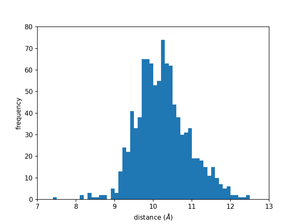
This figure shows the distance distribution and is exactly the same as the one we get in tutorial 4.2.
2.2 2D-Histogram
We then try to analyze the secondary structure data (output.tor) obtained in Tutorial 3.1 and draw a 2D histogram (the Ramachandran plot). As mentioned in section 2.1, there is also more than one method to make a 2D histogram plot. Here, we simply utilize the matplotlib.pyplot.hist2d function.
# Change directory to 2d-histogram analysis
$ cd ../Analysis2.2
$ ls
hist2d.py output.tor
The program can be found in the file hist2d.py:
#!/usr/bin/env python3

import numpy as np
import matplotlib.pyplot as plt

# load data from file (use the 1st and 2nd columns)
x_data, y_data = np.loadtxt("output.tor", usecols=(1, 2), unpack=True)

# plot the 2d histogram with 72 bins on each dimension
plt.hist2d(x_data, y_data, bins=[72, 72], range=[[-180, 180], [-180, 180]], cmap="Reds")

# set aspect ratio to "equal"
plt.gca().set_aspect('equal', 'box')

# set ticks for x and y axis
plt.xticks([-180, -135, -90, -45, 0, 45, 90, 135, 180])
plt.yticks([-180, -135, -90, -45, 0, 45, 90, 135, 180])

# set x and y axis labels
plt.xlabel(r"$\phi$ ($^\circ$)")
plt.ylabel(r"$\psi$ ($^\circ$)")

# plot a color bar
plt.colorbar(label="frequency")

# save figure to file
plt.savefig("Ramachandran_plot.png", dpi=150)
np.loadtxtis used to load data from a file. Here we use the 2nd and 3rd columns of “output.tor” (usecols=(1, 2)) and store them in different arrays (unpack=True).plt.hist2d()is a function that calculates and draws the 2D histogram. We specify the number of bins (72) and range ([-180, 180]) in each dimension, respectively.plt.gca()is a method to “Get the Current Axis”. We then set the aspect ratio of the current axis to “equal” and fix it to the “box”, which generates a square frame of the plot, instead of a rectangle by default.plt.xticks()andplt.yticks()set the ticks of the x and y-axis, respectively.plt.xlabel()andplt.ylabel()set the labels of the x and y-axis, respectively.plt.colorbar()add a color bar to explain the color map of the histogram plot.plt.savefig()saves the current plot to a png file.
By running the following commands in the subdirectory Analysis2.2:
$ ./hist2d.py

# or
$ python3 hist2d.py
we get the figure in the file Ramachandran_plot.png as shown in the following:
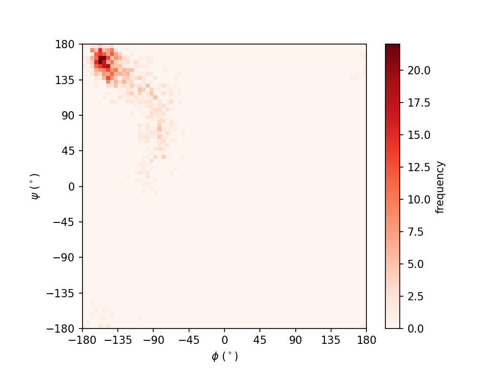
In this figure, the intensity of the red color represents the frequency of the dihedral angle pair (φ, ψ).
Written by Cheng Tan@RIKEN Center for Computational Science, Computational Biophysics Research Team
October, 2021