14.3 Relative protein-ligand binding free energy
Contents
1. Alchemical calculation for relative binding free energy
One of the most important applications of the FEP method is the calculation of protein-ligand binding affinity, which is defined as the free-energy change upon ligand binding to a target protein. Here, we demonstrate how to calculate the relative binding affinity between two ligands to FK506 Binding Protein (FKBP) [1] using the FEP method. The FKBP-ligand system is often used as a benchmark system to estimate the performance of protein-ligand binding affinity calculations [2]. Figure 1 shows the thermodynamic cycle for the binding of FKBP to ligands L8 and L9. The relative binding affinity, \(\Delta\Delta G_{bind}\), is defined as the difference between the absolute binding affinities of two ligands: \(\Delta\Delta G_{bind}=\Delta G_{bind}^{L9}-\Delta G_{bind}^{L8}\). In calculations of absolute binding affinities, the free-energy change from the bound state (the ligand fully interacts with the protein and solvent) to the unbound state (the ligand loses all interactions with the protein and solvent) must be calculated. However, since the perturbation between the bound and unbound states is significantly large, many intermediate states (usually more than 30) are required to keep the statistical error within an acceptable range. As shown in Figure 1, instead of explicitly calculating \(\Delta G_{bind}^{L8}\) and \(\Delta G_{bind}^{L9}\), \(\Delta\Delta G_{bind}\) can be calculated by mutation from L8 to L9 as follows:
\( \displaystyle \Delta\Delta G_{bind} = \Delta G_{mut}^{complex} – \Delta G_{mut}^{ligand},\)
where \(\Delta G_{mut}^{complex}\) and \(\Delta G_{mut}^{ligand}\) are the free energy changes upon mutation from L8 to L9 in the bound and unbound states, respectively. Since the perturbation in the mutation is small (from a benzene ring in L8 (green in Figure 1) to a cyclohexyl ring in L9 (magenta in Figure 1)), the number of intermediate states can be reduced.
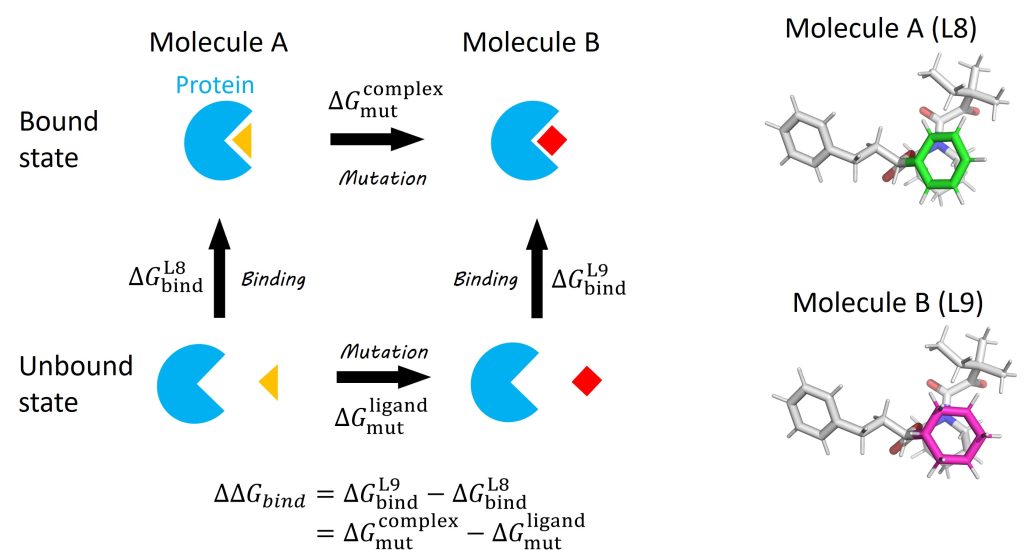
Figure 1. (Left) Thermodynamic cycle of protein-ligand binding and ligand mutation. (Right) Structures of ligands L8 and L9.
Similary to relative solvation free energy calculations, \(\Delta G_{mut}^{complex}\) and \(\Delta G_{mut}^{ligand}\) can be calculated by gradually changing the topology and interactions of the ligand using FEP. However, the environment of the ligand is different for relative solvation and binding. In the relative solvation case, the ligand is in vacuum or in solvent, whereas for relative binding, the ligand is in the binding site of the target protein or in solvent. When in the binding site, the interactions between the protein and the ligand significantly contribute to the binding free energy.
2. System setup
2. 1. Overview of required input files
We will demonstrate FEP calculations of relative binding affinities of the FKBP-ligand systems. First, download the tutorial files (tutorial22-14.3). The tutorial consists of three directories: complex, ligand, and toppar. complex and ligand contain files for FEP simulations of the protein-ligand complex and ligand in water, respectively. toppar contains CHARMM force field parameter files .
# Download the tutorial file$ cd /home/user/GENESIS/Tutorials$ mv ~/Downloads/tutorial22-14.3.zip ./$ unzip tutorial22-14.3.zip$ cd tutorial-14.3$ lscalc_ddG.py* complex/ ligand/ toppar/
# Setup the directory for binary files of GENESIS 1.7.1$ export GENESIS_BIN_DIR=../../../GENESIS_Tutorials-2019/Programs/genesis-1.7.1/bin/
The complex directory contains script files and input files. run_min.inp, run_eq1.inp, run_eq2.inp, and run_eq3.inp are GENESIS control files for minimization, heating, equilibration with restraints, and long equilibration without restraints, respectively. make_inp.sh is a shell script for generating the control file for the production run of FEP simulations. post_run.sh is a shell script for analysis. The ligand directory also contains input files similar to the complex directory.
$ cd complex$ lscomplex.pdb make_input.sh* post_run.sh* run_eq2.inp run_eq.sh* run_min.inpcomplex.psf output/ run_eq1.inp run_eq3.inp run_fepremd.sh*
In this tutorial we will learn how to calculate the relative binding affinity based on the CHARMM force field. However, the calculation can be also performed using the AMBER force field. If you use the AMBER force field, download the tutorial files for the AMBER force field (tutorial22-14.3_amber). The options in the GENESIS control files for the AMBER force field are very similar to the CHARMM force field.
2. 2. Hybrid topology of L8 and L9
Figure 2 shows the hybrid topology of L8 and L9. In GENESIS spdyn, the hybrid-topology structure of L8 and L9 is realized by superimposing the common atoms of the two molecules (i.e., the single-topology part). Since the common atoms are duplicated in the system, spdyn removes the additional degrees of freedom in the duplicated atoms, and always synchronizes their coordinates and velocities during the FEP simulations as if the common part had no duplication.
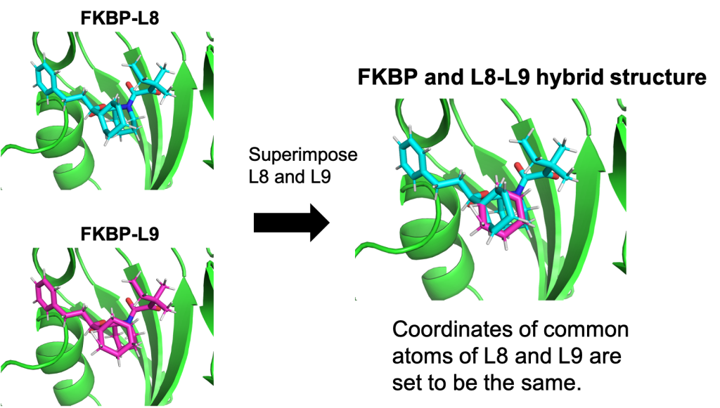
Figure 2. The hybrid topology of L8 and L9.
Figure 3 shows the PDB file for the hybrid topology. The PDB file must contain the coordinates of ligands A and B, followed by those of protein and water. Each ligand is divided into single-topology and dual-topology parts. The single-topology and dual-topology parts of the initial state (L8: segment ID L0) are respectively referred to as “single A” and “dual A”, while those of the final state (L9: segment ID L1) are referred to as “single B” and “dual B”, respectively. The atom names, coordinates, and order of “single A” atoms must be the same as those of the “single B” atoms, because the “single A” and “single B” parts are assumed to be the same in the FEP simulations. The PSF file (or PRMTOP file for AMBER) corresponding to the PDB file is also required for the FEP simulations.
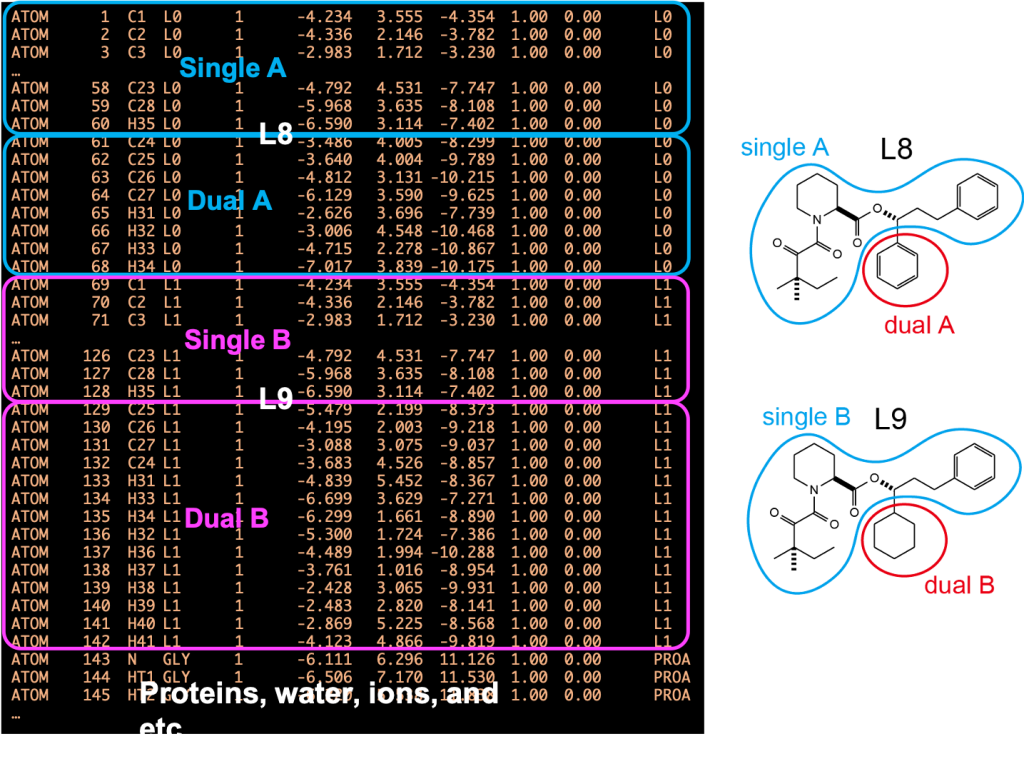
Figure 3. (Left) PDB file for hybrid topology. (Right) Definitions of singleA, singleB, dualA, and dualB.
The PDB and PSF files for hybrid topology can be prepared manually, but the process is troublesome and prone to error. Even a minor difference between the coordinates or the order of “single A” and “single B” atoms will lead to an early termination of the simulation. Instead, creation of input files can be automated using the CHARMM-GUI utility tools (Figure 4). The relative Ligand Binder tool in CHARMM-GUI automatically prepares PDB, PSF, and GENESIS input files for hybrid topology calculations. A ligand can be easily mutated to another ligand of interest using graphical user interface, and force field parameters for the ligands are automatically generated using ParamChem. The PDB and PSF files in tutorial22-14.3.zip were generated using the Relative Ligand Binder tool in CHARMM-GUI.
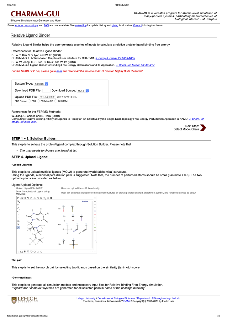
Figure 4. Front page of the Relative Ligand Binder tool in CHARMM-GUI.
3. FEP simulations in the ligand-bound state
3. 1. Minimization and equilibration
Before the production run, we carry out minimization and equilibration of the system with alchemical perturbation. First, we carry out the minimization in order to remove atomic clashes (or bad contacts) in the initial structure. The following command executes the minimization procedure:
# Perform minimization$ $GENESIS_BIN_DIR/spdyn -np 8 run_min.inp > output/run_min.out
The important sections of the minimization control file are shown below. fep_direction, fepout_period, and equilsteps are not used during the minimization, and they can be omitted. In [SELECTION] section, group1, group2, group3, and group4 are respectively assigned to singleA, singleB, dualA, and dualB atoms defined in Figure 3. Here we set all values of lambljA, lambljB, lambelA, lambelB, lambbondA, and lambbondB to 1.0, which means that L8 and L9 molecules fully interact with the other atoms in the system. lambrest can be omitted if the restraint is not scaled by \(\lambda\).
[ALCHEMY]fep_topology = HybridsingleA = 1 # Group number for singleA atomssingleB = 2 # Group number for singleB atomsdualA = 3 # Group number for dualA atomsdualB = 4 # Group number for dualB atomssc_alpha = 5.0sc_beta = 0.5lambljA = 1.0lambljB = 1.0lambelA = 1.0lambelB = 1.0lambbondA = 1.0lambbondB = 1.0[SELECTION]group1 = ai:1-60 and segid:L0 # group for singleA atomsgroup2 = ai:69-128 and segid:L1 # group for singleB atomsgroup3 = ai:61-68 and segid:L0 # group for dualA atomsgroup4 = ai:129-142 and segid:L1 # group for dualB atoms
Next, we heat up the system from 0.1 K to 300 K. The following command executes the heating procedure:
# Perform heating$ $GENESIS_BIN_DIR/spdyn -np 8 run_eq1.inp > output/run_eq1.out
In FEP MD simulations, the energy difference (\(\Delta U\)) between two states is calculated. \(\lambda\) values for each state are specified by a column in lambljA, lambljB, lambelA, lambelB, lambbondA, and lambbondB. In the control file shown below, two columns of \(\lambda\) values correspond to two states. When Forward is specified in fep_direction, GENESIS performs a FEP simulation only at state 1 (left column of \(\lambda\) values) and calculates the energy difference between states 1 and 2 (right column of \(\lambda\) values) at state 1. The energy difference is outputted to fepfile specified in [OUTPUT]. In this example, \(\lambda\) values of states 1 and 2 are identical, therefore the energy difference is 0.
[OUTPUT]dcdfile = output/run_eq1.dcdrstfile = output/run_eq1.rstfepfile = output/run_eq1.fepout[ALCHEMY]fep_direction = Forwardfep_topology = HybridsingleA = 1singleB = 2dualA = 3dualB = 4fepout_period = 0equilsteps = 0sc_alpha = 5.0sc_beta = 0.5lambljA = 1.0 1.0lambljB = 1.0 1.0lambelA = 1.0 1.0lambelB = 1.0 1.0lambbondA = 1.0 1.0lambbondB = 1.0 1.0
Subsequently, we perform NPT equilibration with restraints (100 ps) and NPT equilibration without restraints (1 ns). In those simulations, the [ALCHEMY] section is identical to that of the heating simulation. After the simulations have ended, it is recommended to check the log files and confirm the trajectories using a visualization tool such as VMD.
# Perform equilibration with positional restraints$ $GENESIS_BIN_DIR/spdyn -np 8 input/run_eq2.inp > output/run_eq2.out# Perform equilibration without the restraints$ $GENESIS_BIN_DIR/spdyn -np 8 input/run_eq3.inp > output/run_eq3.out
3. 2. FEP/\(\lambda\) REMD simulations
In this step, we perform the production run of FEP/REMD simulations. To enhance the sampling efficiency, FEP simulations at different \(\lambda\) values are coupled using the Hamiltonian replica exchange method [5,6]. Here, we prepare 12 replicas. The first and the last replicas correspond to the initial and final states, respectively, while the other 10 replicas correspond to intermediate states. 12 replicas run in parallel and exchange their parameters at fixed intervals during the simulation. Exchanges between adjacent replicas are accepted or rejected according to the Metropolis criterion.
The following command generates input files for FEP/REMD simulations:
# Execute the shell script for generation of input files$ sh make_inp.sh
This make_inp.sh script generates five input files (run_fep1.inp to run_fep5.inp). Each file is for a 1-ns FEP/REMD simulation. By executing the scripts sequentially, we obtain a total of a 5-ns simulation. In this tutorial, we use only the run_fep1.inp (i.e., only a 1-ns simulation is performed). If 12 replicas are too large for the user’s computer resources, use the “embarrassingly parallel computing” option by modifying make_inp.sh (see Sec 14.1.6).
The most important sections in run_fep1.inp are shown below. In the FEP/REMD simulation, [REMD] section is also required. type1 is set to alchemy to exchange \(\lambda\) values. exchange_period should be a multiple of fepout_period. In the [ALCHEMY] section, fep_direction is set to BothSides. The \(\lambda\) values for each replica are specified by lambljA, lambljB, lambelA, lambelB, lambbondA, and lambbondB. The leftmost column of the \(\lambda\) values corresponds to the parameters for the initial state (i.e., L8), the rightmost column corresponds to the parameters for the final state (i.e., L9), and the remaining columns correspond to the parameters for the intermediate states. In this tutorial, LJ, electrostatic, and bonded interactions are simultaneously and linearly changed along replica IDs as shown in Figure 5. sc_alpha and sc_beta are the parameters for the LJ and electrostatic soft-core potentials [3,4], respectively. When the LJ and electrostatic interactions are simultaneously changed, the electrostatic soft-core potential is required, because the electrostatic interactions sometimes become very large when the repulsive interaction in LJ are weakened (due to the distance between two atoms becomes too short). Here we set sc_beta to 5.0.
[REMD]dimension = 1exchange_period = 800type1 = alchemynreplica1 = 12[ALCHEMY]fep_direction = BothSidesfep_topology = hybridsingleA = 1singleB = 2dualA = 3dualB = 4fepout_period = 400equilsteps = 0sc_alpha = 5.0sc_beta = 5.0lambljA = 1.0 0.909 0.818 0.727 0.636 0.545 0.455 0.364 0.273 0.182 0.091 0.0lambljB = 0.0 0.091 0.182 0.273 0.364 0.455 0.545 0.636 0.727 0.818 0.909 1.0lambelA = 1.0 0.909 0.818 0.727 0.636 0.545 0.455 0.364 0.273 0.182 0.091 0.0lambelB = 0.0 0.091 0.182 0.273 0.364 0.455 0.545 0.636 0.727 0.818 0.909 1.0lambbondA = 1.0 0.909 0.818 0.727 0.636 0.545 0.455 0.364 0.273 0.182 0.091 0.0lambbondB = 0.0 0.091 0.182 0.273 0.364 0.455 0.545 0.636 0.727 0.818 0.909 1.0lambrest = 1.0 1.0 1.0 1.0 1.0 1.0 1.0 1.0 1.0 1.0 1.0 1.0
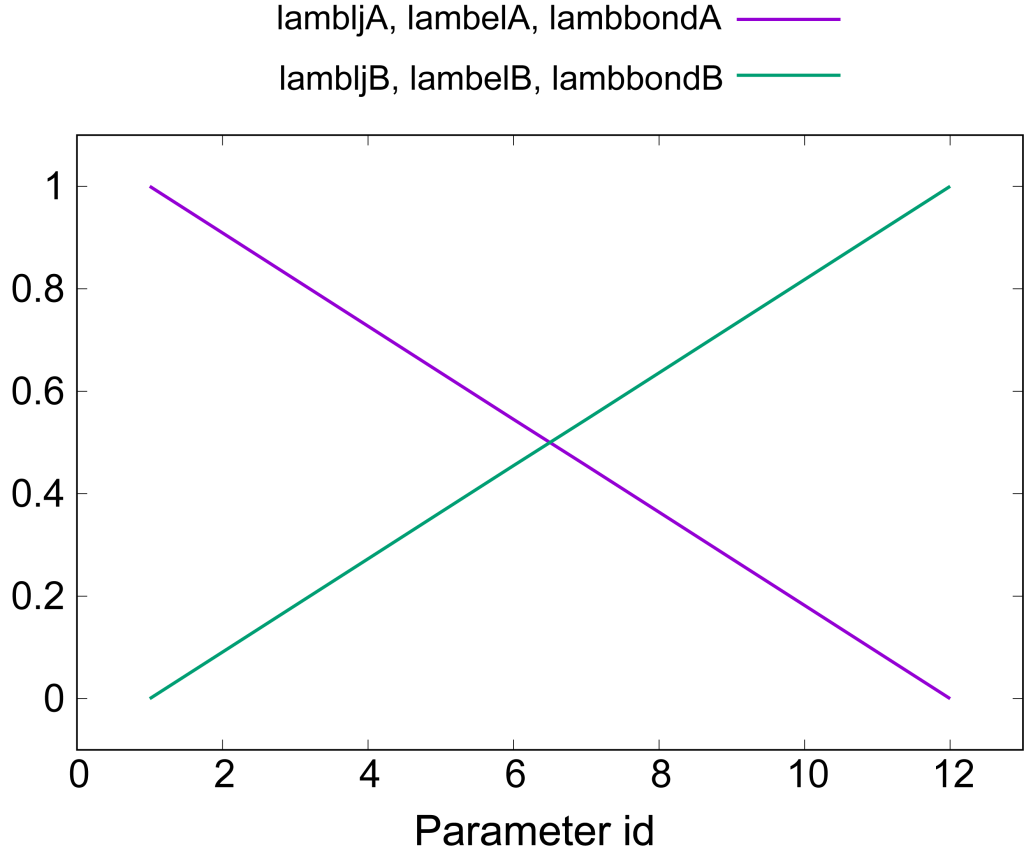
Figure 5. Values of [latex]\lambda[/latex] for electrostatic, LJ, and bonded interactions.
The following command executes the FEP/\(\lambda\)REMD simulation:
# Execute the control file for the lambda-exchange FEP simulation# 8 MPI processes per replica, i.e. 8 * 12 = 96 processes are used here$ $GENESIS_BIN_DIR/spdyn -np 96 input/run_fep1.inp > output/run_fep1.out
For the purpose of this tutorial, we here perform only a 1-ns FEP/\(\lambda\)REMD simulation using the r-RESPA integrator with 2.5-fs time step. However, this might not be sufficient for convergence of the free-energy calculation. For obtaining more accurate results, it is recommended to use a longer simulation time, in accoradnace with the computational resources or time available to the user.
3. 3. Analysis
After the FEP/\(\lambda\)REMD simulation have ended, we calculate the free energy from the fepfile file. The post_run.sh script calculates the free-energy difference between the initial and final states:
# Execute the shell script for analysis$ sh post_run.sh
In the first part of the post_run.sh script, fepfile files are sorted using remd_convert and energy differences for each parameter (par1.fepout to par12.fepout) are written. In the second part, the free-energy differences between the reference state (state A = L8) and the target state (state B = L9) are calculated using mbar_analysis in GENESIS analysis tools. Finally, post_run.sh outputs a file named fene.dat (Figure 6). By default, the trajectories are divided into three blocks, and each column in fene.dat represents the free-energy changes in each block (i.e., the block average of the free-energy changes are obtained). Each row represents the free-energy change from the initial state (state A = L8). The last row corresponds to the free-energy change from the initial state to the final state (state B = L9), which is equal to \(\Delta G_{mut}^{complex}\).
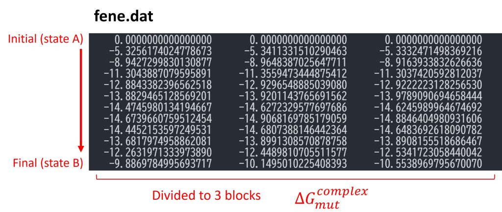
Figure 6. Free-energy changes from the initial state to the final state in the bound state.
4. FEP simulations in the ligand-unbound state
Next, we perform simulations in the unbound state for obtaining \(\Delta G_{mut}^{ligand}\) (change directory to ligand). We consider a system which includes only the ligand and solvent molecules, because the protein does not affect the free-energy change upon ligand mutation (see Figure 1). Namely, the calculation of \(\Delta G_{mut}^{ligand}\) corresponds to that of \(\Delta G_{mut}^{solvent}\) of L8 and L9, which is shown in Sec.14.1. Input files are very similar to those for FEP simulations described in Sec.14.1 with minor differences. After performing minimization, equilibration, and FEP/REMD simulations, we can obtain \(\Delta G_{mut}^{ligand}\) by executing post_run.sh.
5. Comparison with the experimental value
Figure 7 shows the free-energy changes from the initial state (L8: Parameter ID 1) to the final state (L9: Parameter ID 12). The difference between the initial and final states for the protein-ligand complex and that for the isolated ligand in water correspond to \(\Delta G_{mut}^{complex}\) and \(\Delta G_{mut}^{ligand}\), respectively. From our calculations, we obtained \(\Delta G_{mut}^{complex}=−10.20±0.19 \)kcal/mol and \(\Delta G_{mut}^{ligand} =−10.05±0.19 \)kcal/mol. Therefore, the relative binding affinity of L8 and L9 is \(\Delta G_{bind} =−0.15±0.27\) kcal/mol, which is in good agreement with the experimental results (0.2 kcal/mol) [1].
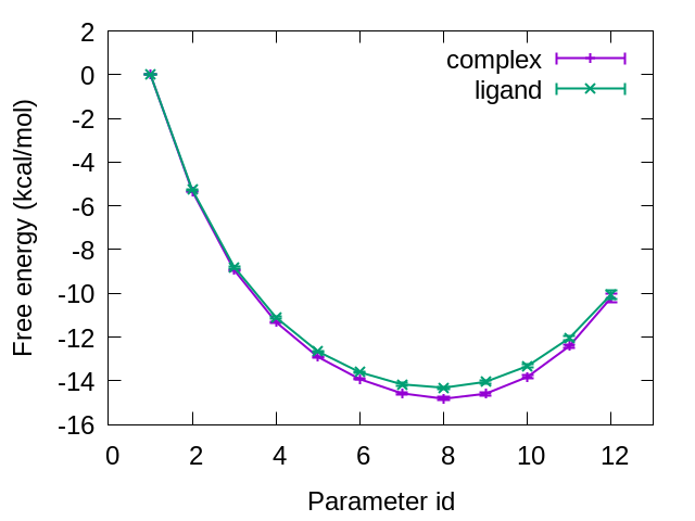
Figure 7. Free-energy changes from the initial state to the final state for complex and ligand.
6. References
- D. A. Holt, J. I. Luengo, D. S. Yamashita, H. J. Oh, A. L. Konialian, H. K. Yen, L. W. Rozamus, M. Brandt, M. J. Bossard, Design, Synthesis, and Kinetic Evaluation of High-Affinity FKBP Ligands and the X-Ray Crystal Structures of Their Complexes with FKBP12. J. Am. Chem. Soc. 115, 9925–9938 (1993).
- H. Fujitani, Y. Tanida, and A. Matsuura, Massively parallel computation of absolute binding free energy with well-equilibrated states. Phys. Rev. E 79, 021914 (2009).
- M. Zacharias, T. P. Straatsma, and J. A. McCammon, Separation‐shifted scaling, a new scaling method for Lennard‐Jones interactions in thermodynamic integration. J. Chem. Phys. 100, 9025–9031 (1994).
- T. Steinbrecher, I. Joung, and D. A. Case, Soft-core potentials in thermodynamic integration: Comparing one- and two-step transformations. J. Comput. Chem. 32, 3253–3263 (2011).
- Y. Sugita, A. Kitao, and Y. Okamoto, Multidimensional Replica-Exchange Method for Free-Energy Calculations. J. Chem. Phys. 113, 6042–6051 (2000).
- H. Fukunishi, O. Watanabe, S. Takada, On the Hamiltonian Replica Exchange Method for Efficient Sampling of Biomolecular Systems: Application to Protein Structure Prediction. J. Chem. Phys. 116, 9058−9067 (2002)
Written by Hiraku Oshima@RIKEN BDR
March 31, 2022