14.1 Relative solvation free energy
Contents
In this tutorial, we will briefly introduce the free-energy perturbation (FEP) method and demonstrate how to calculate the relative solvation free energy of two solutes using FEP functions implemented in GENESIS.
1. Introduction
1. 1. Free-energy perturbation (FEP)
The free-energy difference between two states, A and B, can be estimated by the following statistical thermodynamics relation:
\( \displaystyle \Delta G = G_B – G_A \\ \displaystyle= – k_BT \ln \frac{\int dx \exp[-\beta U_B(x)]}{\int dx \exp[-\beta U_A](x)} \\ \displaystyle = – k_BT \ln \frac{\int dx \exp[-\beta U_A (x)- \beta \Delta U(x)]}{\int dx \exp[-\beta U_A(x)]} \\ \displaystyle = – k_BT \ln \left<\exp[-\beta \Delta U(x)]\right>_A,\)
where G and U are the free energy and potential energy of state A or B, and \( \Delta U\) is the difference between UA and UB. According to this equation, \( \Delta G\) can be estimated by sampling only equilibrium configurations of state A and calculating the “perturbation”, hence this method is called “free-energy perturbation (FEP)”.
However, if the difference between states A and B is large (i.e., the perturbation is too large), there is little overlap between the energy distributions (left of Figure 1) and the configurations at state B are poorly sampled by simulations in state A, leading to large statistical errors. To reduce such errors, n−2 intermediate states are inserted between states A and B in order to obtain overlapped energy distributions (right of Figure 1). The potential energy of intermediate state i is defined by
\( \displaystyle U(\lambda_i) = (1-\lambda_i)U_A + \lambda_i U_B\),
where λi is the scaling parameter coupling the initial and final states. By changing λi from 0 to 1, states A and B can be smoothly connected. \( \Delta G\) can be estimated by calculating the summation of free-energy changes between adjacent states:
\( \displaystyle \Delta G = \sum_{i=0}^{n-1} \Delta G_i \displaystyle= – k_BT \sum_{i=0}^{n-1} \ln \left<\exp[-\beta (U(\lambda_{i+1}) – U(\lambda_i)) \right>_{\lambda_i},\),
where the subscript λi represents the ensemble average at state i. Since the free energy depends only on the initial and final states, any configuration of intermediate states can be chosen, regardless of whether or not the states are physically realizable. If the intermediate states are physically unrealizable but computationally realizable, the calculation and thermodynamic process are referred to as alchemical free-energy calculation and alchemical process, respectively.
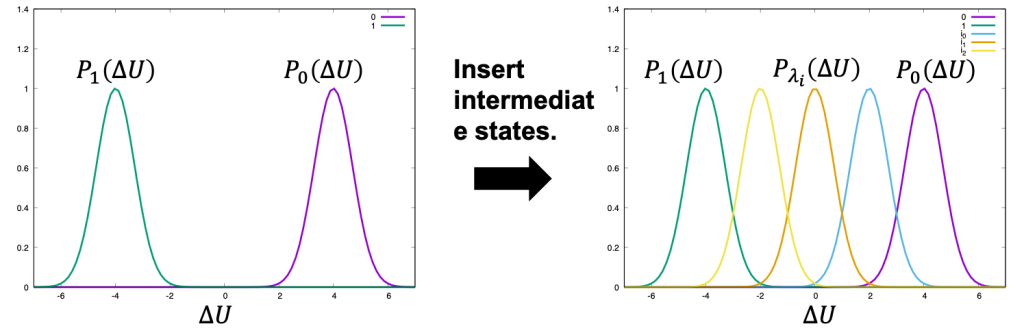
Figure 1. Distribution of energy differences.
1. 2 Relative solvation free energy
Using an alchemical processes, the FEP method can be applied to the calculation of solvation free energies of solutes. The relative solvation free energy \(\Delta \Delta G_{solv}\) is defined as the difference between the absolute solvation free energies of two solutes: \(\Delta \Delta G_{solv} = \Delta G_{solv}^{B} – \Delta G_{solv}^{A}\). In calculations of absolute solvation free energies, the free-energy change upon the transfer of the solute from vacuum (= the solute does not interact with any other molecules) to the solvent (= the solute interacts with water molecules) must be calculated. In general, since all the interactions of the ligand are included in the perturbation, many intermediate states are required to keep the statistical error within an acceptable range. In contrast, from the thermodynamic cycle shown in Figure 2, \(\Delta \Delta G_{solv}\) can be calculated by mutation from A to B (instead of calculating absolute solvation free energies): \(\Delta \Delta G_{solv}=\Delta G_{mut}^{solvent}- \Delta G_{mut}^{vacuum}\), where \(\Delta G_{mut}^{solvent}\) and \(\Delta G_{mut}^{vacuum}\) are the free energy changes upon mutation from A to B in solvent and vacuum, respectively. Since the perturbation accompanying the mutation is small (from a hydrogen atom of benzene to an OH group of phenol (right of Figure 2)), the number of intermediate states can be reduced, thus reducing the total error in the calculation.
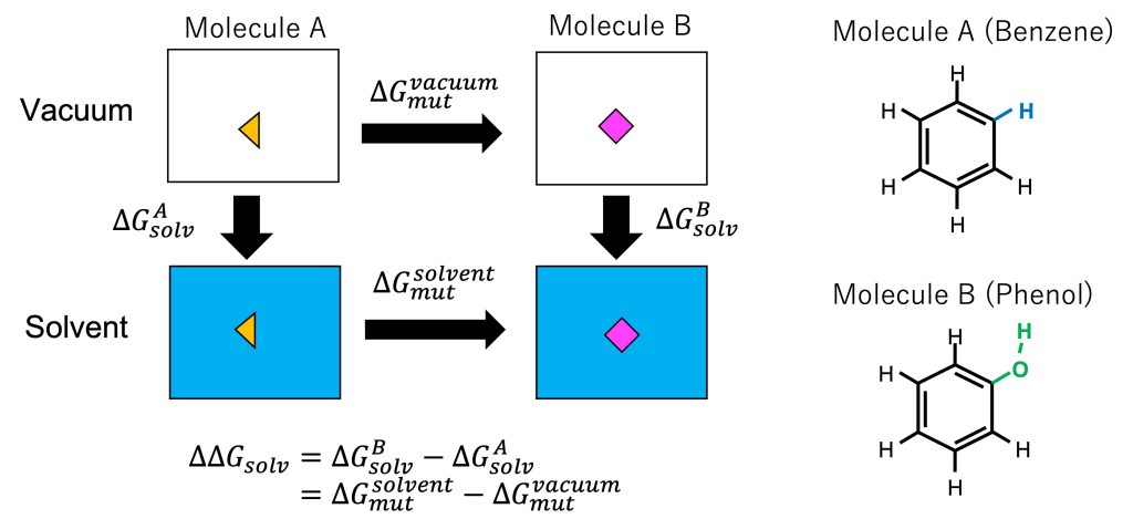
Figure 2. (Left) Thermodynamic cycle for calculating the solvation free energy and mutation of solute. (Right) Molecules A and B.
1. 3. Hybrid-topology approach
In order to mutate from benzene to phenol, we must consider the differences in topologies and force field parameters between the two molecules. For the case of benzene and phenol shown in Figure 2. the two molecules have a common part (the benzene ring and five hydrogen atoms) and a different part (H atom for benzene and OH group for phenol). The common parts share the same topology but they differ in their charge distribution as well as in the parameters for bonds, angles, and dihedrals. The different atoms (H for benzene and OH for phenol) differ in both their topology and force field parameters. In order to account for the difference between the systems, we introduce the “hybrid topology approach” [1,2,3] to FEP simulations. In this approach, we set them up such that the common part has a single topology, while the different parts have a dual topology (Figure 3). Each part is hereafter referred to as the single-topology or dual-topology part, respectively.
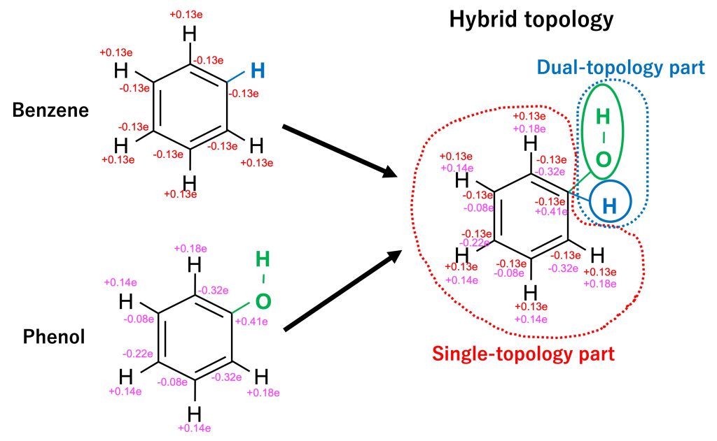
Figure 3. The topologies of benzene and phenol are merged into a hybrid topology.
During the FEP simulation, the topology of the single-topology part is not changed, but its force field parameters (charge, LJ, and internal bond) are gradually changed from state A to state B. In the dual-topology part, both topologies and parameters are changed. In order to smoothly connect states A and B, in the hybrid topology approach, the potential energy is modified by lambda values (\(\lambda_{LJ}^{A}, \lambda_{LJ}^{B}, \lambda_{elec}^{A}, \lambda_{elec}^{B}, \lambda_{bond}^{A}, \lambda_{bond}^{B}\)) which gradually change from state A to state B. At the initial state corresponding to state A, only the H atom of benzene exists in the dual-topology part and the force field parameters correspond to those of benzene, while in the final state corresponding to state B, only the OH atoms exist in the dual-topology part and the force field parameters correspond to those of phenol (Figure 4).
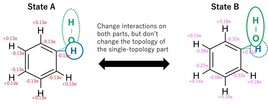
Figure 4. The alchemical transformation from benzene to phenol using the hybrid topology approach.
1. 4. Soft-core potentials
In the vicinity of the initial and the final states (\(\lambda_{LJ}^{A}, \lambda_{LJ}^{B}\) = 0 or 1), overlap between perturbed atoms or between perturbed and non-perturbed atoms can lead to drastic energy changes. A situation in which the simulation becomes unstable due to such overlaps is termed “end point catastrophe” and can lead to an early termination of the simulation. In order to avoid such a situation, soft-core potential is introduced to the LJ potential [4]. In GENESIS, in additon to the LJ potential, the soft-core potential is applied to the electrostatic potentials [5]. The formulas of the soft-core potentials are shown in GENESIS Users’ Manual.
1. 5. Functions available in GENESIS
GENESIS supports several types of alchemical calculations. Functions implemented in GENESIS include hybrid and dual-topology calculation methods, soft-core potentials, and lambda-exchange calculations based on REMD. In addition, acceleration of FEP simulations is possible using GPGPU. Currently, SPDYN supports only the CHARMM and AMBER force fields for FEP simulations. FEP functions are only available in GENESIS version 1.x.x. GENESIS 2.0 does not support FEP yet. Full description of the available functions is provided in the users’ manual. In this tutorial, we demonstrate the usage of FEP functions in GENESIS by calculating the relative solvation free energy between methane and methanol.
2. System setup
2. 1. Overview of required input files
We will perform FEP simulations for obtaining the relative solvation free energy of methane and methanol. First, download the tutorial files (tutorial22-14.1). The tutorial consists of two directories: methane-methanol and toppar. The methane-methanol directory includes ligand and vacuum directories, which contain input files for performing FEP simulations in solvent and in vacuum, respectively. The toppar directory contains CHARMM force field parameter files.
# Download the tutorial file$ cd /home/user/GENESIS/Tutorials$ mv ~/Downloads/tutorial22-14.1.zip ./$ unzip tutorial22-14.1.zip$ cd tutorial-14.1$ lsmethane-methanol/ toppar/$ cd methane-methanol$ lsREADME calc_ddG.py ligand/ vacuum/# Setup the directory for binary files of GENESIS 1.7.1$ export GENESIS_BIN_DIR=../../../GENESIS_Tutorials-2019/Programs/genesis-1.7.1/bin/
The ligand directory contains script files and input files for calculating \(\Delta G_{mut}^{solvent}\). run_min.inp, run_eq1.inp, run_eq2.inp, and run_eq3.inp are GENESIS control files for minimization, heating, equilibration with restraints, and equilibration without restraints, respectively.
make_inp.sh is a shell script for generating control file for the production run of FEP simulations. post_run.sh is a shell script for analysis. The vacuum directory contains respective input files for calculatiing \(\Delta G_{mut}^{vacuum}\).
$ cd ligand$ lsrun_eq.sh* ligand.psf output/ run_eq2.inp run_fep2.inprun_fepremd.sh* make_input.sh* post_run.sh* run_eq3.inp run_min.inpligand.pdb make_job.sh* run_eq1.inp run_fep1.inp
2. 2. Structure files for the hybrid-topology approach
To treat hybrid topology in GENESIS, the common parts of methane and methanol (i.e., the single-topology part) are superimposed, meaning that common atoms are duplicated (Figure 5). The duplication introduces unnecessary degrees of freedom, and an error may occur if coordinates and velocities of common atoms become different for the two systems. In GENESIS, those additional degrees of freedom are removed, and the coordinates and velocities of the common atoms are synchronized throughout the FEP simulations.
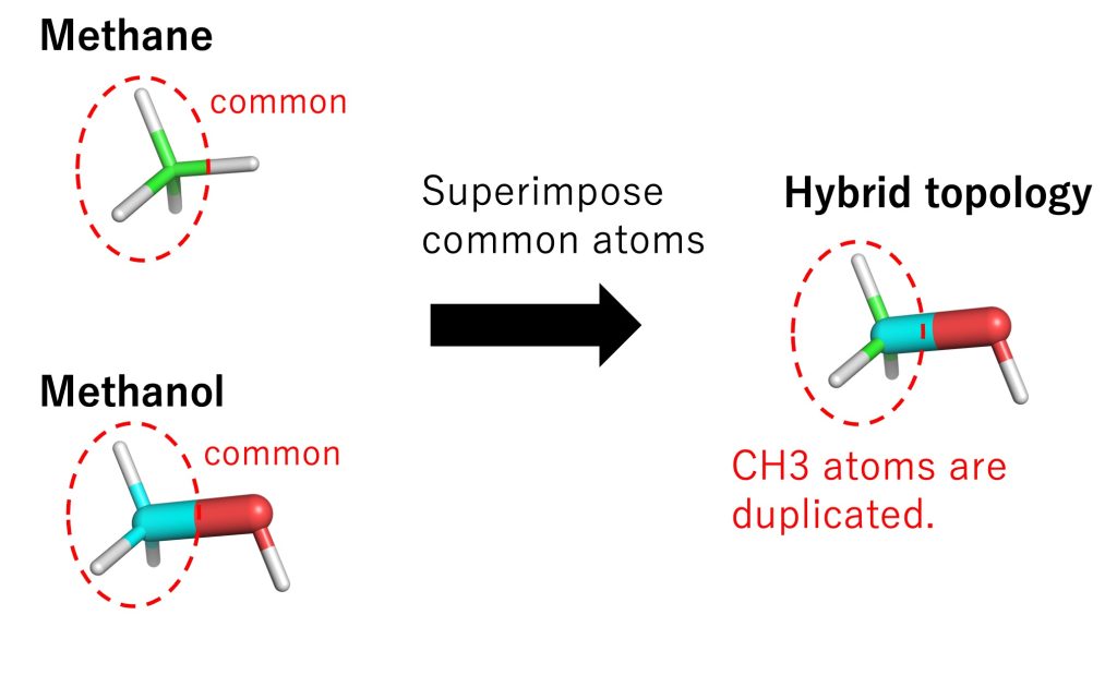
Figure 5. Representation of hybrid topology in GENESIS
An section of the PDB file is shown in Figure 6. The PDB file must contain the coordinates for all atoms of solutes A (methane) and B (methanol). Each solute is divided into single-topology and dual-topology parts. The single-topology and dual-topology parts of the initial state (methane: segment ID L0) are respectively referred to as “singleA” and “dualA”, while those of the final state (methanol: segment ID L1) are referred to as “singleB” and “dualB”, respectively. The atom names, coordinates, and order of “singleA” atoms must be identical to those of the “singleB” atoms, because the “singleA” and “singleB” parts are treated as such in the FEP simulations. The PSF file corresponding to the PDB file is also required.
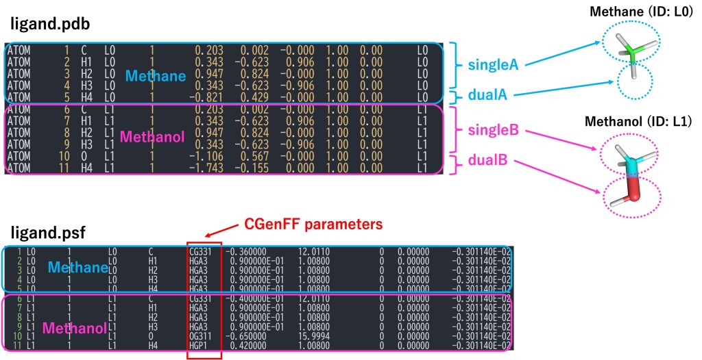
Figure 6. PDB and PSF files for the hybrid topology and definitions of singleA, singleB, dualA, and dualB.
The PDB and PSF files for the hybrid-topology approach can be prepared manually, but the process is troublesome and prone to error. Even a minor difference between the coordinates or the order of “single A” and “single B” atoms will lead to an early termination of the simulation. Instead, creation of input files can be automated using the CHARMM-GUI utility tools. The relative Ligand Solvator tool in CHARMM-GUI automatically prepares PDB, PSF, and GENESIS input files for hybrid-topology approach calculations. A solute can be easily mutated to another using graphical user interface, and force field parameters for solutes are automatically generated using ParamChem. The input files in tutorial22-14.1.zip were generated by the CHARMM-GUI Relative Ligand Solvator tool. However, some files were modified for the purpose of this tutorial.
2. 3. The ALCHEMY section
Most input options in the GENESIS control file are identical to the ones used in Tutorial 3.2, but here, the [ALCHEMY] section was added to set the keywords related to FEP. To see available input options for the [ALCHEMY] section, execute the following command:
# Show control options$ $GENESIS_BIN_DIR/spdyn -h ctrl_all md
The output of the command is shown below. fep_direction represents the direction of energy evaluation in FEP. BothSides, Forward, or Reverse are available. The topology in FEP simulations is specified by fep_topology (Hybrid or Dual). For hybrid topology, fep_topology = Hybrid is set. The “singleA”, “singleB”, “dualA”, and “dualB” atoms of the ligands are assigned by the keywords: singleA, singleB, dualA, and dualB, respectively. For these keywords, we set the group numbers assigned in [SELECTION]. For example, if group1, group2, group3, and group4 are respectively assigned to singleA, singleB, dualA, and dualB atoms in [SELECTION] section, then we set singleA = 1, singleB = 2, dualA = 3, and dualB = 4. fepout_period is the frequency of output of energy difference. It must be larger than or equal to eneout_period. equilsteps represents the number of equilibration steps performed before the evaluation of energy differences. In GENESIS, soft-core potentials are applied to the LJ [5] and electrostatic [6] interactions between the dual-topology atoms and the others. sc_alpha and sc_beta are the parameters of the soft-core potentials for LJ and electrostatic interactions, respectively. lambljA, lambljB, lambelA, lambelB, lambbondA, lambbondB, and lambrest represent values of \(\lambda\) for LJ, electrostatics, internal bonds, and restraints, respectively.
# [ALCHEMY]# fep_direction = Bothsides # Fep direction [Bothsides, Forward, Reverse]# fep_topology = Hybrid # Fep topology [Hybrid, Dual]# fep_md_type = Serial # FEP-MD or FEP-REMD [Serial, Single, Parallel]# singleA = 1 # Group number for singleA atoms# singleB = 2 # Group number for singleB atoms# dualA = 3 # Group number for dualA atoms# dualB = 4 # Group number for dualB atoms# fepout_period = 100 # output period for energy difference# equilsteps = 0 # number of equilibration steps# sc_alpha = 5.0 # LJ soft-core parameter# sc_beta = 0.5 # Electrostatic soft-core parameter# lambljA = 1.0 0.75 0.5 0.25 0.0 # lambda for LJ in region A# lambljB = 0.0 0.25 0.5 0.75 1.0 # lambda for LJ in region B# lambelA = 1.0 0.75 0.5 0.25 0.0 # lambda for electrostatic in region A# lambelB = 0.0 0.25 0.5 0.75 1.0 # lambda for electrostatic in region B# lambbondA = 1.0 0.75 0.5 0.25 0.0 # lambda for internal bonds in singleA# lambbondB = 0.0 0.25 0.5 0.75 1.0 # lambda for internal bonds in singleB# lambrest = 1.0 1.0 1.0 1.0 1.0 # lambda for restraint energy# ref_lambid = 0 # Reference window id for single FEP-MD
3. FEP simulations in solvent
3. 1. Minimization and equilibration
We carry out minimization and equilibration of the system with alchemical perturbation before the production run. First, we carry out the minimization in order to remove atomic clashes (or bad contacts) in the initial structure. The following command executes the minimization procedure:
# Perform minimization$ $GENESIS_BIN_DIR/spdyn -np 8 run_min.inp > output/run_min.out
The important sections of the minimization control file are shown below. fep_direction, fepout_period, and equilsteps are not used during the minimization, and they can be omitted. In the [SELECTION] section, group1, group2, group3, and group4 are respectively assigned to singleA, singleB, dualA, and dualB atoms defined in Figure 6. We here set lambljA and lambljB to 1.0, denoting that methane and methanol have full LJ interactions with the other atoms in the system. Also, we set lambelA, lambelB, lambbondA, and lambbondB to 0.5. lambrest is set to 1.0, but it can be omitted if the restraint is not scaled by \(\lambda\). The soft-core parameters for LJ and electrostatic interactions are set to 5.0.
[ALCHEMY]fep_topology = HybridsingleA = 1 # Group number for singleA atomssingleB = 2 # Group number for singleB atomsdualA = 3 # Group number for dualA atomsdualB = 4 # Group number for dualB atomssc_alpha = 5.0sc_beta = 5.0lambljA = 1.0lambljB = 1.0lambelA = 0.5lambelB = 0.5lambbondA = 0.5lambbondB = 0.5lambrest = 1.0[SELECTION]group1 = ai:1-4 and segid:L0 # group for singleA atomsgroup2 = ai:6-9 and segid:L1 # group for singleB atomsgroup3 = ai:5-5 and segid:L0 # group for dualA atomsgroup4 = ai:10-11 and segid:L1 # group for dualB atoms
Next, we heat up the system from 0.1 K to 300 K. The following command executes the heating procedure:
# Perform heating$ $GENESIS_BIN_DIR/spdyn -np 8 run_eq1.inp > output/run_eq1.out
In FEP MD simulations, the energy difference (\(\Delta U\)) between two states is calculated. \(\lambda\) values for each state are specified by a column in lambljA, lambljB, lambelA, lambelB, lambbondA, and lambbondB. In the control file shown below, two columns of \(\lambda\) values correspond to two states. When ‘Forward’ is specified in fep_direction, GENESIS performs a FEP simulation only at state 1 (left column of \(\lambda\) values) and calculates the energy difference between states 1 and 2 (right column of \(\lambda\) values) at state 1. The energy difference is outputted to ‘fepfile’ specified in [OUTPUT]. In this example, \(\lambda\) values of states 1 and 2 are identical, therefore the energy difference is 0. fepout_period and equilsteps should be specified, but these values are not used during the equilibration.
[OUTPUT]dcdfile = output/run_eq1.dcdrstfile = output/run_eq1.rstfepfile = output/run_eq1.fepout[ALCHEMY]fep_direction = Forwardfep_topology = HybridsingleA = 1singleB = 2dualA = 3dualB = 4fepout_period = 0equilsteps = 0sc_alpha = 5.0sc_beta = 0.5lambljA = 1.0 1.0lambljB = 1.0 1.0lambelA = 0.5 0.5lambelB = 0.5 0.5lambbondA = 0.5 0.5lambbondB = 0.5 0.5
Subsequently, we perform NPT equilibration with restraints (100 ps) and NPT equilibration without restraints (100 ps). In those simulations, the [ALCHEMY] section is identical to that of the heating simulation. After the simulations have ended, it is recommended to check the log files and confirm the trajectories using a visualization tool such as VMD.
# Perform equilibration with positional restraints$ $GENESIS_BIN_DIR/spdyn -np 8 input/run_eq2.inp > output/run_eq2.out# Perform equilibration without the restraints$ $GENESIS_BIN_DIR/spdyn -np 8 input/run_eq3.inp > output/run_eq3.out
3. 2. FEP/\(\lambda\) REMD simulations
In this step, we perform the production run of the FEP simulations. To enhance the sampling efficiency, FEP simulations at different \(\lambda\) values are coupled using the Hamiltonian replica exchange method [6,7]. Here, we prepare 12 replicas. The first and the last replicas correspond to the initial and final states, respectively while the other 10 replicas correspond to intermediate states. 12 replicas run in parallel and exchange their parameters at fixed intervals during the simulation. Exchanges between adjacent replicas are accepted or rejected according to the Metropolis criterion.
We execute two 1-ns FEP/REMD simulations (run_fep1.inp and run_fep2.inp) sequentially for a total of a 2-ns simulation. Input files for sequential runs can be easily generated by the following command:
# Execute the shell script for generation of input files
$ sh make_inp.sh
The simulation time can be modified in the “make_inp.sh” script (5-ns by default).
The most important sections in run_fep1.inp are shown below. In the FEP/\(\lambda\)REMD simulation, [REMD] section is also required. type1 is set to alchemy, meaning that \(\lambda\) values are exchanged. exchange_period should be a multiple of fepout_period. nreplica1 specifies the number of replicas. In the [ALCHEMY] section, fep_direction is set to BothSides. When BothSides is specified, the energy differences between adjacent replicas are calculated for each replica, i.e., for replica i, the energy differences between i and i-1 and between i and i+1 are calculated and written to the file specified by fepfile at the fixed intervals specified by fepout_period. In Figure 7, fepfile is shown for replica 3 (window 3). The fepfile files are used to calculate the free energy in the next section “3.3. Analysis”. The \(\lambda\) values for each replica are specified by lambljA, lambljB, lambelA, lambelB, lambbondA, and lambbondB. The leftmost column of the \(\lambda\) values corresponds to the parameters for the initial state (i.e., methane), the rightmost column corresponds to the parameters for the final state (i.e., methanol), and the remaining columns correspond to the parameters for the intermediate states. In this tutorial, we linearly change lambljA, lambljB, lambelA, lambelB, lambbondA, and lambbondB along replica IDs, as shown in Figure 8.
[REMD]dimension = 1exchange_period = 800type1 = alchemynreplica1 = 12[ALCHEMY]fep_direction = BothSidesfep_topology = hybridsingleA = 1singleB = 2dualA = 3dualB = 4fepout_period = 400equilsteps = 0sc_alpha = 5.0sc_beta = 5.0lambljA = 1.0 0.909 0.818 0.727 0.636 0.545 0.455 0.364 0.273 0.182 0.091 0.0lambljB = 0.0 0.091 0.182 0.273 0.364 0.455 0.545 0.636 0.727 0.818 0.909 1.0lambelA = 1.0 0.909 0.818 0.727 0.636 0.545 0.455 0.364 0.273 0.182 0.091 0.0lambelB = 0.0 0.091 0.182 0.273 0.364 0.455 0.545 0.636 0.727 0.818 0.909 1.0lambbondA = 1.0 0.909 0.818 0.727 0.636 0.545 0.455 0.364 0.273 0.182 0.091 0.0lambbondB = 0.0 0.091 0.182 0.273 0.364 0.455 0.545 0.636 0.727 0.818 0.909 1.0lambrest = 1.0 1.0 1.0 1.0 1.0 1.0 1.0 1.0 1.0 1.0 1.0 1.0
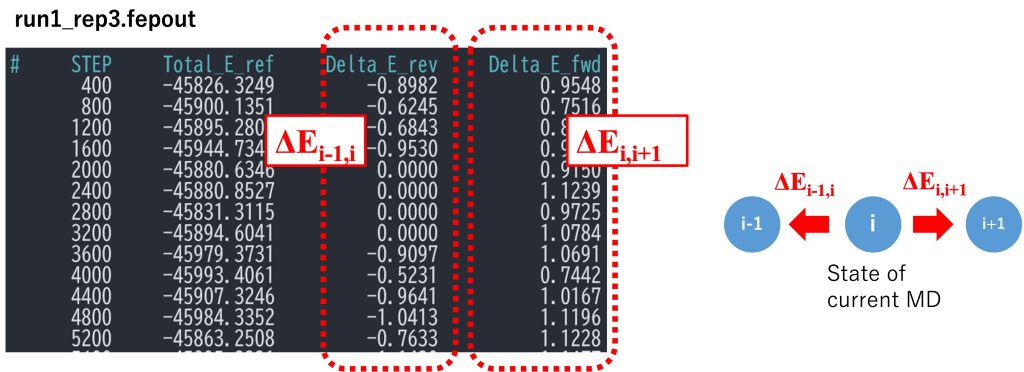
Figure 7. Example of fepfile.
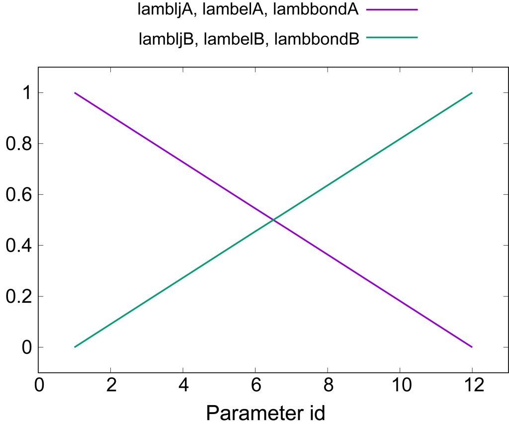
Figure 8. Values of lambda for electrostatic, LJ, and bonded interactions.
The following command executes the FEP/\(\lambda\)REMD simulation:
# Execute the control file for the lambda-exchange FEP simulation# 8 MPI processes per replica, i.e. 8 * 12 = 96 processes are used here$ $GENESIS_BIN_DIR/spdyn -np 96 input/run_fep1.inp > output/run_fep1.out
We perform a FEP/\(\lambda\)REMD simulation using the r-RESPA integrator with a 2.5-fs time step. Here, the length of the simulation is 2 ns, which might not be sufficient for the convergence the free-energy calculation. For obtainning more accurate results, it is recommended to use a longer simulation time, in accordance with the computational resources or time available to the user.
3. 3. Analysis
After the FEP/\(\lambda\)REMD simulations have ended, we calculate the free energy from fepfile. The post_run.sh script calculates the free-energy difference between the initial and final states:
# Execute the shell script for analysis$ sh post_run.sh
In the first part of the post_run.sh script, fepfile files are sorted using remd_convert and energy differences for each parameter are outputted (par1.fepout to par12.fepout). remd_convert is included in GENESIS analysis tools. In the second part, the free-energy differences between adjacent parameter sets are calculated from the sorted files using the Bennett acceptance ratio (BAR) method [8] (the relevant section of the post_run.sh script is shown below). The BAR method is performed using mbar_analysis in GENESIS analysis tools. The number of simulations, number of replicas, number of steps, frequency of replica exchange, frequency of energy output, and the temperature are specified by nrun, nrep, nsteps, exchange_period, fepout_period, and temperature, respectively. These parameters can be adapted according to the user’s system.
# set parameters of simulationsnrun=2nrep=12nsteps=400000exchange_period=800fepout_period=400temperature=300
Finally, post_run.sh outputs a file named “fene.dat” (Figure 9), which includes the free-energy differences along the parameter IDs. By default, the trajectories are divided tino three blocks, and each column in fene.dat represents the free-energy changes in each block (i.e., the block average of the free-energy changes are obtained). Each row represents the free-energy change from the initial state (state A). The last row corresponds to the free-energy change from the initial state to the final state (state B), which is equal to \(\Delta G_{mut}^{solvent}\).
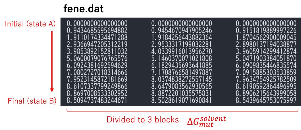
Figure 9. Free-energy changes from the initial state to the final state in the solvent.
4. FEP simulations in vacuum
Next, we perform FEP simulations in vacuum to obtain \(\Delta G_{mut}^{vacuum}\) . Please change directory to “vacuum”. Input files for the vacuum simulations are very similar to those for the solvent simulations, but there are some important differences described as follows. There are no water molecules in vacuum.pdb and vacuum.psf. In run_min.inp, run_eq[1-3].inp, and run_fep[1-2].inp, vacuum option is set to “YES”. CUTOFF is used for energy evaluation instead of PME. The cutoff distance should be set to a sufficiently large value (here we use 300Å). The box size should be consistent with the large pairlist distance. Also, NVT should be used in order to fix the simulation box size. If NPT is used in a vacuum simulation, the box size shrinks drastically, which can lead to an early termination of the simulation.
[ENERGY]forcefield = CHARMM # [CHARMM]electrostatic = CUTOFF # [CUTOFF,PME]switchdist = 298.0 # switch distancecutoffdist = 300.0 # cutoff distancepairlistdist = 305.0 # pair-list distancevdw_force_switch = YESvacuum = YES[BOUNDARY]type = PBC # [PBC]box_size_x = 921box_size_y = 921box_size_z = 921
Similarly to FEP simulations in solvent, after performing minimization, equilibration, and FEP/\(\lambda\)REMD simulations, we can obtain \(\Delta G_{mut}^{vacuum}\) by executing post_run.sh.
5. Calculation of \(\Delta \Delta G_{solv} \) and comparison with the experimental value
Figure 10 shows the free-energy changes from the initial state (methane) to the final state (methanol). The free-energy change in window ID 12 for “in solvent” and “in vacuum” corresponds to \(\Delta G_{mut}^{solvent} \) and \(\Delta G_{mut}^{vacuum} \), respectively. From our calculations, we obtained \(\Delta G_{mut}^{solvent} = 8.52±0.01 \) kcal/mol and \(\Delta G_{mut}^{vacuum} = 15.35±0.00 \) kcal/mol. Therefore, the relative solvation free energy is \(\Delta \Delta G_{solv} = −6.83±0.01 \) kcal/mol, which is in good agreement with the experimental value (-7.10 kcal/mol [9]).
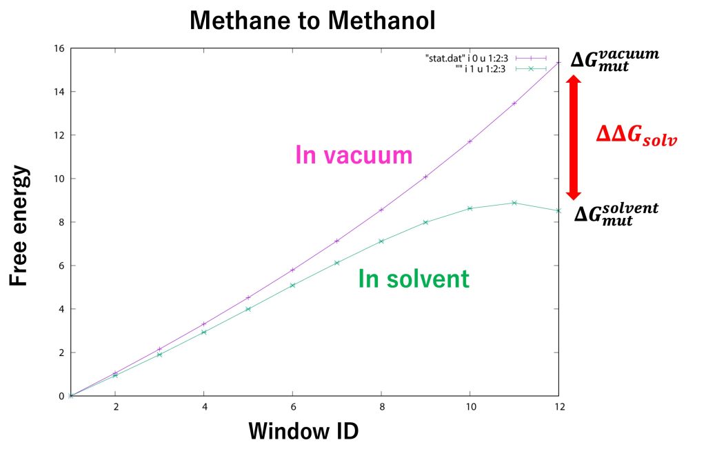
Figure 10. Free-energy changes from the initial state to the final state for “in solvent” and “in vacuum”.
6. (Optional) Embarrassingly parallel computing
FEP/\(\lambda\)REMD requires large computational resources at one time, because MD simulations for all \(\lambda\) windows must be performed simultaneously in order to be exchanged periodically. However, if replica-exchange is not used, \(\lambda\) windows are independent from each other, and simulations for different \(\lambda\) values can be performed separately. This parallelization scheme is called “embarrassingly parallel” (also called “bakapara” in Japanese). To generate input files for embarrassingly parallel FEP simulations, comment out md_type=remd and uncomment md_type=distributed in make_inp.sh.
# set md type (remd or distributed)#md_type=remdmd_type=distributed
make_inp.sh generates 60 input files (run1_rep1.inp to run1_rep12.inp, run2_rep1.inp to run2_rep12.inp, …). run1_rep1.inp is an input file for performing a 1-ns FEP simulation for window ID 1 only. A section of the run1_rep1.inp file is shown below. In this input file, [REMD] section is removed. fep_md_type and ref_lambid are added in [ALCHEMY] section. When fep_md_type is set to Single, the simulation uses only one lambda window and becomes embarrassingly parallel. ref_lambid specifies the lambda windows used for the simulation.
[ALCHEMY]fep_direction = BothSidesfep_topology = hybridfep_md_type = Singleref_lambid = 1singleA = 1singleB = 2dualA = 3dualB = 4...
MD simulations for different replicas run1_rep1.inp to run1_rep12.inp can be executed independently. Input files for different run numbers (i.e., run2_rep*.inp, run3_rep*.inp, …) are executed sequentially to obtain a 5-ns simulation in total.
In embarrassingly parallel computation, there is no need to sort the fepfile file using remd_convert. To obtain the free-energy difference, comment out md_type=remd and uncomment md_type=distributed in post_run.sh to avoid sorting and to concatenate fepfile obtained by FEP simulations, respectively.
7. References
- J. W. Kaus, L. T. Pierce, R. C. Walker, and J. A. McCammon, Improving the Efficiency of Free Energy Calculations in the Amber Molecular Dynamics Package. J. Chem. Theory Comput. 9, 4131–4139 (2013).
- W. Jiang, C. Chipot, and B. Roux, Computing Relative Binding Affinity of Ligands to Receptor: An Effective Hybrid Single-Dual-Topology Free-Energy Perturbation Approach in NAMD. J. Chem. Inf. Model. 59, 3794–3802 (2019).
- S. Kim, H. Oshima, H. Zhang, N. R. Kern, S. Re, J. Lee, B. Roux, Y. Sugita, W. Jiang, W. Im, CHARMM-GUI Free Energy Calculator for Absolute and Relative Ligand Solvation and Binding Free Energy Simulations, J. Chem. Theory Comput., 16, 7207-7218 (2020).
- M. Zacharias, T. P. Straatsma, and J. A. McCammon, Separation‐shifted scaling, a new scaling method for Lennard‐Jones interactions in thermodynamic integration. J. Chem. Phys. 100, 9025–9031 (1994).
- T. Steinbrecher, I. Joung, and D. A. Case, Soft-core potentials in thermodynamic integration: Comparing one- and two-step transformations. J. Comput. Chem. 32, 3253–3263 (2011).
- Y. Sugita, A. Kitao, and Y. Okamoto, Multidimensional Replica-Exchange Method for Free-Energy Calculations. J. Chem. Phys. 113, 6042–6051 (2000).
- H. Fukunishi, O. Watanabe, S. Takada, On the Hamiltonian Replica Exchange Method for Efficient Sampling of Biomolecular Systems: Application to Protein Structure Prediction. J. Chem. Phys. 116, 9058−9067 (2002).
- C. H. Bennett, Efficient estimation of free energy differences from Monte Carlo data, J. Comput. Phys. 22, 245-268 (1976)
-
D. L. Mobley, J. P. Guthrie, FreeSolv: A Database of Experimental and Calculated Hydration Free Energies, with Input Files, J. Comput. Aided Mol. Des. 28, 711–720 (2014).
Written by Hiraku Oshima@RIKEN BDR
February 22, 2022