12.5 Gaussian accelerated Replica-Exchange Umbrella Sampling (GaREUS)
Contents
- Preparation
- 1. Equilibration
- 2. Production run of GaREUS
- 3. Analysis
- 3.1 Remove water molecules from trajectories
- 3.2 Sort trajectories and log files by parameters of REUS
- 3.3 Calculate end-to-end distances
- 3.4 Reweight REUS biases using MBAR
- 3.5 Reweight GaMD biases using the cumulant expansion
- 3.6 Calculate dihedral angles
- 3.7 Reweight the free-energy landscape of the dihedral angles
- References
Biomolecules have many local-minimum energy states and the transition between the states are very slow (e.g., 1 \(\mu\)s to 1 ms). Since conventional MD simulations often get trapped at local-minimum states, it is difficult to capture conformational changes related to the biomolecular functions within the accessible computational time. To overcome this difficulty, enhanced-sampling methods based on collective variables (CVs) are often used in biomolecular simulations. In these methods, one or two CVs are employed to represent the conformational change, and biases are applied in the CV space to enhance conformaional sampling. For example, in Replica-Exchange Umbrella Sampling method (REUS[1,2]), restraint potentials along the CVs are exchanged between replicas to search the CV space. However, the determination of CVs requires expert knowledge about the biosystems. If the choice of CVs is wrong, the convergence of the free-energy calculation becomes very slow.
To further improve the sampling efficiency, two different types of enhanced sampling methods are combined. One is a CV-based method, while another is a CV-free method. Recently, we proposed the combination of REUS with Gaussian accelearated MD (GaMD) [3,4], which is called Gaussian accelerated REUS (GaREUS) [5]. In the method, the boost potential of GaMD \(\Delta U^{\text{GaMD}}\) and the restraint poteintal of REUS \(\Delta U_i^{\text{REUS}}\) are added to the system potential:
\( \displaystyle U”(x) = U(x)+\Delta U^{\text{GaMD}}\left(U(x)\right) + \Delta U_i^{\text{REUS}}\left(\xi(x)\right),\)
where \(x\) is the configuration of the system, \(U\) is the potential energy of the system, \(i\) is the replica ID, \(\xi(x)\) is the CV, and the double prime represents the biased value. REUS enhances sampling along the CV space, while GaMD accelerates the molecular flexiblity or dynamics by adding a boost potential to the system (Figure 1). The boost potentials in GaMD lower the hidden energy barriers existing in the orthogonal degrees of freedom for the CV spaces used in REUS, resulting in faster convergence for free-energy calculation in GaREUS compared to REUS, while keeping a similar computational cost.
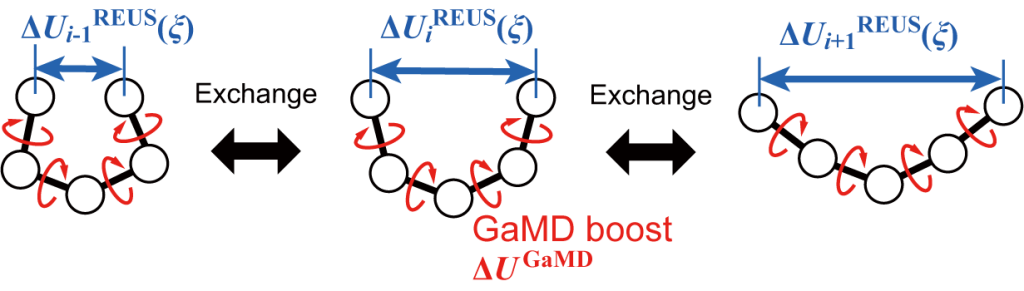
Figure 1. Scheme of GaREUS.
In this tutorial, we demonstrate a GaREUS simulation of a trialanine (Ala)3 by applying GaMD into REUS simulations in tutorial 12.2.
Preparation
First of all, let’s download the tutorial file (tutorial22-12.5). This tutorial consists of seven steps: 1) system setup, 2) minimization and equilibration, 3) determination of initial parameters of GaMD by a short simulation, 4) determination of GaMD parameters with updating, 5) equilibration at each replica, 6) production run of GaREUS, and 7) trajectory analysis. However, Steps 1 to 4 are common to Tutorial 12.4. We reuse the results of GaMD simulations by making symbolic links to tutorial-12.4. Please finish tutorial 12.4 before you start the GaREUS tutorial.
# Download the tutorial file $ cd ~/GENESIS_Tutorials-2022/Works$ mv ~/Download/tutorial22-12.5.zip ./$ unzip tutorial22-12.5.zip$ rm tutorial22-12.5.zip$ cd tutorial-12.5$ ls5_equilibration 6_production/ 7_analysis/# Make a symbolic link to the CHARMM toppar directory$ ln -s ../../Data/Parameters/toppar_c36_jul21 ./toppar# Make symbolic links to the directory in tutorial-12.4$ ln -s ../tutorial-12.4/1_setup .$ ln -s ../tutorial-12.4/4_update_parameter .# Setup the directory for binary files of GENESIS 2.0$ export GENESIS_BIN_DIR=../../../GENESIS_Tutorials-2022/Programs/genesis-2.0/bin/
If you skip tutorial 12.4, the restart file for next calculations are not included in the tutorial file. Please download tutorial22-12.5_full, which includes “1_setup” and “4_update_parameter” directories.
1. Equilibration
In tutorial 12.4 we have already determined the GaMD parameters of (Ala)3 in water. Here we reuse the prameters for GaREUS simulations without any changes. First, we carry out equilibration of REUS replicas with applying GaMD boost potentials. Let’s move to the directory for equilibration.
# Change directory for equilibration
$ cd 5_equilibration
$ ls
run.sh  run.inp
run.inp is the control file for equilibration of GaREUS. The part of its content is shown below.
[GAMD] gamd = yes boost = yes boost_type = DUAL thresh_type = LOWER sigma0_pot = 6.0 sigma0_dih = 1.0 update_period = 0 pot_max = -37468.2812 pot_min = -38756.9062 pot_ave = -37715.0977 pot_dev = 80.5305 dih_max = 23.1753 dih_min = -3.0486 dih_ave = 11.8922 dih_dev = 2.3506[REMD]dimension = 1exchange_period = 0type1 = RESTRAINTnreplica1 = 14cyclic_params1 = NOrest_function1 = 1
...[SELECTION]group1 = an:OY and resno:1 # restraint group 1group2 = an:HNT and resno:3 # restraint group 2[RESTRAINTS]nfunctions = 1function1 = DISTconstant1 = 1.2 1.2 1.2 1.2 1.2 1.2 1.2 1.2 1.2 1.2 1.2 1.2 1.2 1.2reference1 = 1.80 2.72 3.64 4.56 5.48 6.40 7.32 8.24 9.16 10.08 11.00 11.92 12.84 13.76select_index1 = 1 2
This control file represents that the same GaMD biases are applied to each replica of REUS. In the [GAMD] section, the parameters are the same as used in the prodcution run in tutorial 12.4. The dual boost approach is used, and sigma0_pot and sigma0_dih are set to 6 and 1, respectively, for the highest boosting and accurate reweighting. In the [REMD], [SELECTION], and [RESTRAINTS] sections, the setting values are the same as used in the equilibration in tutorial 12.2. The distance restraints are applied to the distance between the OY atom of residue 1 and the HNT atom of residue 3 in (Ala)3. 14 replicas with reference distances (1.8 to 13.76) are not exchanged in the stage of the equlibration (i.e., exchange_period = 0).
Perform a 1-ns NVT GaREUS simulation without replica exchange for equilibration by executing the following command.
# Perform 1-ns GaREUS for equilibration
# 14 replicas * 8 MPI processes per each replica = 112 MPI processes in total
$ $GENESIS_BIN_DIR/spdyn -np 112 run.inp > run.out
Since GaREUS requires large computational cost, we recommend you perform GaREUS simulations on PC clusters or super computers. When you have job submission system on your PC cluster or super computer, Please modify the above command for your enviroment.
2. Production run of GaREUS
Next, we perform 10-ns production run of GaREUS. Let’s move to the directory for production.
$ cd ../6_production $ lsrun.inp run.sh
run.inp is the control file for production of GaREUS.
[REMD]dimension = 1exchange_period = 1250type1 = RESTRAINTnreplica1 = 14cyclic_params1 = NOrest_function1 = 1
...[DYNAMICS]integrator = VVER # Velocity Verlet integratornsteps = 2500000 # number of MD steps (10 ns)timestep = 0.004 # timestep (4 fs)eneout_period = 50 # energy output period (200 fs)crdout_period = 50 # coordinates output period (200 fs)rstout_period = 25000 # restart output periodnbupdate_period = 5 # nonbond update periodthermostat_period = 5 # period of thermostat updatebarostat_period = 5 # period of barostat updatehydrogen_mr = yeshmr_target = Solutehmr_ratio = 2.5hmr_ratio_xh1 = 2.0
The velocity Verlet integrator with the 4-fs time step is used with the HMR and group T/P methods. Replicas are exchanged every 1250 time step (= 5 ps). To reweight the GaMD trajectory with high accuracy, energy and trajectories are frequently outputted (eneout_period = 50 and crdout_period = 50).
Perform a 10-ns NVT GaREUS simulation by executing the following command.
# Perform 10-ns production GaREUS
$ $GENESIS_BIN_DIR/spdyn -np 112 run.inp > run.out
3. Analysis
3.1 Remove water molecules from trajectories
We first remove all water molecules from the trajectory files and superimpose (Ala)3 of each snapshot onto the initial structure. Please move to the analysis directory and execute run.sh. This script file performs crd_convert to each trajectory.
# Change directory
$ cd ../7_analysis/1_convert_dcd
$ ls
run.sh

# Run crd_convert for each trejectory
$ bash ./run.sh
3.2 Sort trajectories and log files by parameters of REUS
We sort the trajectories and log files by REUS’s parameters using remd_convert. Please move to 2_sort_dcd and execute run.sh.
# Change directory $ cd ../2_sort_dcd $ ls run.sh# Run remd_convert to sort trajectories $ bash ./run.sh
GENESIS log files contains the values of GaMD biases, which should be also sorted. Procedures in 3.1 and 3.2 are the same as those in 5.1 and 5.2 in tutorial 12.2. The acceptance ratio and random walk in the parameter space should be checked like 5.3 and 5.3 in tutorial 12.2
3.3 Calculate end-to-end distances
To obtain the free-energy landscape of the end-to-end distance of (Ala)3, we extract the end-to-end distance from the sorted trajectories. Please move to 3_calc_dist and execute run.sh. This script calculates the distance between the OY atom of residue 1 and the HNT atom of residue 3, which is used as the CV for GaREUS.
# Change directory$ cd ../3_calc_dist$ lsrun.sh# Calculate the end-to-end distance$ bash ./run.sh
3.4 Reweight REUS biases using MBAR
The trajectories sorted above are imposed by the REUS biases (restraint) and the GaMD biases (dihedral and potential boosts). To obtain the unbiased free-energy landscape, we should remove the two biases from the trajectories. We here follow the two-step reweighting procedure [5]: reweighting of the GaMD biases after reweghting of the REUS biases.
We first reweight the REUS biases using the multi-state Bennett acceptance ratio (MBAR) method. MBAR provides the unbiased probability for each snapshot:
\( \displaystyle p'(x_{jn}) = \frac{1}{c} \frac{\exp [-\beta U'(x_{jn})]}{\sum_k N_k \exp [\beta (f_k – U”_k(x_{jn}))]},\)
where \(x_{jn}\) is a configureation of snapshot \(n\) at replica \(j\), \(f_k\) is the free energy of replica \(k\), and \(c\) is a normalization constant. The prime of \(p’\) and \(U’\) represent that they are still biased by the GaMD biases.
Let’s move to the directory for reweighting and execute run.sh.
# Change directory$ cd ../4_mbar$ lsrun.sh# Perform MBAR$ bash ./run.sh
run.sh applies mbar_analysis to the trajectories of the end-to-end distance. The control file for mbar_analysis is shown below.
[INPUT]cvfile = ../3_calc_dist/cv{}.dat # Collective variable file[OUTPUT]fenefile = output.fene # free energy filepmffile = output.pmf # potential of mean force fileweightfile = output{}.weight # weight file[MBAR]nreplica = 14input_type = CVdimension = 1nblocks = 1temperature = 300.0target_temperature = 300.0rest_function1 = 1grids1 = 0.0 14.0 141output_unit = kcal/mol[RESTRAINTS]constant1 = 1.2 1.2 1.2 1.2 1.2 1.2 1.2 1.2 1.2 1.2 1.2 1.2 1.2 1.2reference1 = 1.80 2.72 3.64 4.56 5.48 6.40 7.32 8.24 9.16 10.08 11.00 11.92 12.84 13.76is_periodic1 = NO
ouptput.pmf is the free-energy landscape of the end-to-end distance, but it is still biased by the GaMD biases. The weight files (output1.weight to output14.weight) contain \(p'(x_{jn})\). An example of output3.weight is shown below.
\(p'(x_{35})\) corresponds to the fifth line in1 3.695691824266203E-0072 3.701943139577103E-0073 6.002131994695485E-0074 7.978031494587585E-0075 3.705625740677231E-0076 3.550182207698960E-0077 3.791755019587222E-0078 3.706008741906196E-0079 3.705544551952881E-007
...
output3.weight. The weight files will be used in the next reweighting.
3.5 Reweight GaMD biases using the cumulant expansion
The GaMD biases can be reweighted by following equations:
\( \displaystyle p(\xi) = \left<\exp[\beta \Delta U^{\text{GaMD}}]\right>’_{\xi} \frac{p'(\xi)}{\left<\exp[\beta \Delta U^{\text{GaMD}}]\right>’}.\)
\(\left<\exp[\beta \Delta U^{\text{GaMD}}]\right>’_{\xi} \) and \(p'(\xi)\) can be calculated using \(p'(x_{jn})\) (= weight files obtaind by mbar_analysis). However, similar to tutorial 12.4, the slow convergence of \(\left<\exp[\beta \Delta U^{\text{GaMD}}]\right>’_{\xi} \) causes the large statistical error. To reduce the statistical error, the cumulant expansion to the second order are applied to the term [6].
To reweight the GaMD biases, let’s move to 5_reweight_dist.
We here reweight the free-energy landscape of the end-to-end distance. Let’s move to the directory for reweighting.
$ cd ../5_reweight_dist$ lscalc_pmf_1d.py plot.sh run.sh
run.sh is the script for the reweighting. In run.sh, we merge CV trajectories into one file.
## Get CV trajectories$ cp /dev/null cv.dat$ for i in {1..14}; do$ cat ../3_calc_dist/cv${i}.dat >> cv.dat$ done
We extract the GaMD biases from the GENESIS log files, which are sorted in 3.2.
## Get boost potentials from GENESIS log files
$ cp /dev/null out.dat
$ for i in {1..14}; do
$    grep "^INFO" ../2_sort_dcd/par${i}.out >> out.dat
$ done
We merge weight files into one file.
## Get weight from mbar_analysiscp /dev/null weight.datfor i in {1..14}; docat ../4_mbar/output${i}.weight >> weight.datdone
From cv.dat, out.dat, and weight.dat, we can obtain the reweighted free-energy landscape by the following commands.
$ python ./calc_pmf_1d.py -t 300.0 -c 10.0 -n 1000000 --Xmin 0.0 --Xmax 14.0 --Xdel 0.5 --cv_file cv.dat --out_file out.dat --weight_file weight.dat --anharmcalc_pmf_1d.py reweights the free-energy landscape using the cumulant expansion and outputs the unbiased free energies in each bin, “pmf_1d.dat“. weight.dat can be assigned by “--weight_file“. Other options of calc_pmf_1d.py are explained in 7.2 of tutorial 12.4.
The reweighted free-energy landscape is shown in Figure 2. We can see that the free-energy barriers in the unreweighted PMF (i.e., GaMD-biased PMF) becomes lower than those in the reweighted PMF.
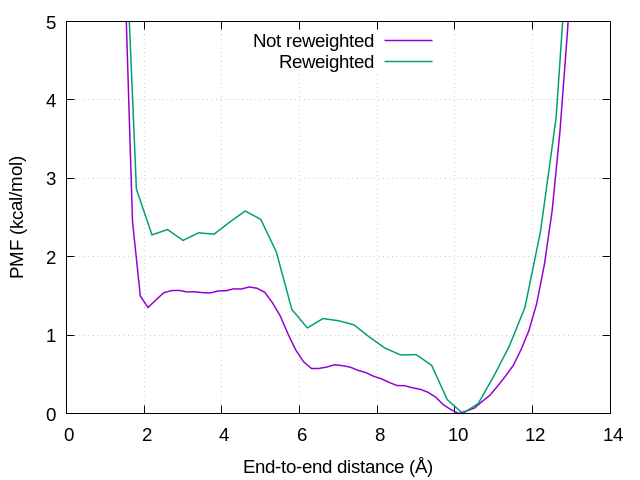
Figure 2. Free-energy landscapes of the end-to-end distance of (Ala)3. Purple and green lines represent unreweighted and reweighted free energies, respectively.
3.6 Calculate dihedral angles
We calculate dihedral angles around residue 2 in (Ala)3. Let’s move to the directory for analysis.
$ cd ../6_calc_dihe$ lsrun.sh
run.sh calculates Φ (torsion 1) and Ψ (torsion 2) dihedral angles from the sorted trajectories. (par1.dcd to par10.dcd in 2_sort_dcd). The values of the dihedrals are outputted to CV files (cv1.dat to cv10.dat).
Execute run.sh to obtain trajectories of dihedrals.
$ bash ./run.sh3.7 Reweight the free-energy landscape of the dihedral angles
To reweight the free-energy landscape of the dihedrals, move to the directory for reweighting.
$ cd ../7_reweight_dihe$ lscalc_pmf_2d.py plot_2d.py plot_anharm.py run.sh
run.sh is the script for the reweighting. In run.sh, we merge CV trajectories, extract the GaMD biases, and merge weght files:
## Get CV trajectories$ cp /dev/null cv.dat$ for i in {1..14}; do$ cat ../6_calc_dihe/cv${i}.dat >> cv.dat$ done## Get boost potentials from GENESIS log files$ cp /dev/null out.dat$ for i in {1..14}; do$ grep "^INFO" ../2_sort_dcd/par${i}.out >> out.dat$ done## Get weight from mbar_analysiscp /dev/null weight.datfor i in {1..14}; docat ../4_mbar/output${i}.weight >> weight.datdone
From cv.dat, out.dat, and weight.dat, we can obtain the reweighted free-energy landscape using calc_pmf_2d.py.
$ python ./calc_pmf_2d.py -t 300.0 -c 10.0 -n 1000000 --Xmin -180.0 --Xmax 180.0 --Xdel 20.0 --Ymin -180.0 --Ymax 180.0 --Ydel 20.0 --cv_file cv.dat --out_file out.dat --weight_file weight.dat --Xcyclic --Ycyclic --anharm$ python ./plot_2d.py
calc_pmf_2d.py reweights the two-dimensional free-energy landscape using the cumulant expansion. weight.dat can be assigned by “--weight_file“. Other options of calc_pmf_2d.py are explained in 7.4 of tutorial 12.4.
plot_pmf_2d.py draws the two-dimensional free-energy landscape using “pmf_2d.dat“, “xi.dat“, and “yi.dat” (Figure 3, Left).
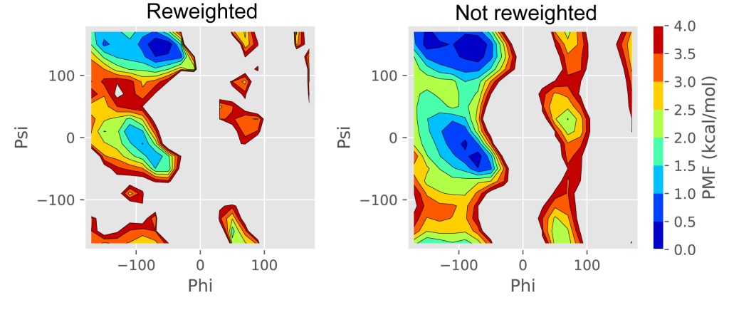
Figure 3. The reweighted and unreweighted free-energy landscapes of two dihedral angles of (Ala)3.
You can also obtain the free-energy landscape without reweighting according to the following commands.
$ python ./calc_pmf_2d.py -t 300.0 -c 10.0 -n 1000000 --Xmin -180.0 --Xmax 180.0 --Xdel 20.0 --Ymin -180.0 --Ymax 180.0 --Ydel 20.0 --cv_file cv.dat --out_file out.dat --weight_file weight.dat --Xcyclic --Ycyclic --noreweightIn the unreweighted free-energy landscape (Figure 3. Right), due to the GaMD biases, the populations of the αR and C7ex conformations are overestimated, while the β/C5 conformation is underestimated. We can confirm that these overestimation and underestimations are modified in the above reweighting.
References
- Y. Sugita, A. Kitao, and Y. Okamoto, J. Chem. Phys. 113, 6042 (2000).
- H. Hukunishi, O. Watanabe, and S. Takada, J. Chem. Phys. 116, 9058 (2002).
- Y. Miao, V. A. Feher, and J. A. McCammon, J. Chem. Theory Comput. 11, 3584–3595 (2015).
- Y. T. Pang, Y. Miao, Y. Wang, and J. A. McCammon, J. Chem. Theory Comput. 13, 9–19 (2017).
- H. Oshima, S. Re, and Y. Sugita, J. Chem. Theory Comput. 15, 5199 (2019).
- Y. Miao, W. Sinko, L. Pierce, D. Bucher, R. C. Walker, and J. A. McCammon, J. Chem. Theory Comput. 10, 2677–2689 (2014).
Written by Hiraku Oshima@RIKEN BDR
June 2, 2022