GENESIS

7.1 Coarse-grained MD simulation with the KB Go-model

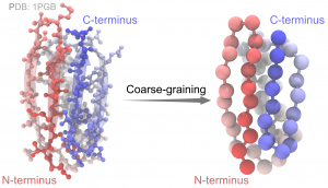
Coarse-grained models are useful for studying large-scale conformational dynamics of biomolecules with time scales that are difficult for atomistic MD simulations to access. Here, we give a simple example of using the coarse-grained model in GENESIS. We are going to simulate the folding/unfolding of protein G, using a variation of the Go-model potential energy function developed by Karanicolas and Brooks [1,2] (hereafter referred to as the KB Go-model).

Please download the tutorial files and extract the tar-ball into your working directory:

# Download the tutorial file
$ cd /home/user/GENESIS/Tutorials
$ mv ~/Downloads/tutorial19-7.1.zip ./
$ unzip tutorial19-7.1.zip
$ cd tutorial-7.1
$ ls
1_construction 2_production 3_analysis

# verify the initial PDB structure 
$ cd 1_construction 
$ vmd 1pgb.pdb 

This tutorial consists of three steps:

1. system setup,
2. production run,
3. trajectory analysis.

1. Setup the system

The KB Go-model simplify each amino acid residue as one coarse-grained bead, which locates at the position of the alpha carbon (Cα). The potential energy function is given in section 5.1 of the GENESIS manual. There are differences between the KB Go-model and a typical atomistic model:

1. no electrostatic terms in the KB Go-model;
2. the vdW terms are divided into two terms: native contacts and non-native contacts, where the native contacts have 12-10-6-type attractive potential, while the non-native contacts have 12-type repulsive potential.

In the first step, we are going to generate a param file (parameter file) and a top file (topology file) by using the MMTSB web service. After this, we are going to use VMD to create a psf file (protein structure file) that is required for GENESIS simulation.

To build a simulation system, we start from downloading a PDB file of protein G from the RCSB Protein Data Bank (also can be found in 1_construction/1pgb.pdb). You can download the PDB file via a web browser, or use the following commands:

# change to the construction directory
$ cd /path/to/1_construction

# download the PDB file (PDB code 1PGB)
$ wget https://files.rcsb.org/download/1PGB.pdb

The downloaded PDB file has to be “cleaned” by removing everything except the lines starting with the ATOM flag:

# "clean" the file by deleting the entries other than ATOM
$ grep -e "^ATOM" 1PGB.pdb > 1pgb_edited.pdb

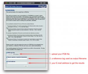
Then we submit it to the MMTSB server:

1. upload our “cleaned” PDB file (1_construction/1pgb_edited.pdb);
2. give a reference tag (i.e. 1pgb);
3. enter your e-mail address.

The webpage looks like this:

After MMTSB finishes the calculations, a tar-ball will be sent to your email address (we provided one as 1_construction/1pgb.tar). Extract the tar-ball into the working directory and you will find the coarse-grained coordinate, topology and parameter files.

# extract the tar-ball file
$ tar xvf /path/to/1pgb.tar

Here we only simulate a single-chain protein. However, if the protein of interest contains multiple chains, you have to manually modify the BOND, ANGLE, DIHEDRAL and NBFIX parameters in the *.param files. Besides, “Bond CA + CA” information in the *.top files should also be corrected. After these modifications, the topology and interactions of the whole structure should be visually verified in VMD.

A VMD script (1_construction/setup.tcl) is provided to build the GO model below:

##### read pdb
mol load pdb GO_1pgb.pdb

##### replace residue names with G1, G2, G3, ...
set all [atomselect top all]
set residue_list [lsort -unique [$all get resid]]
foreach i $residue_list {
    set resname_go [format "G%d" $i]
    set res [atomselect top "resid $i" frame all]
    $res set resname $resname_go
}

$all writepdb tmp.pdb

##### generate PSF and PDB files
package require psfgen
resetpsf
topology GO_1pgb.top

segment PROT {
 first none
 last none
 pdb tmp.pdb
}
regenerate angles dihedrals
coordpdb tmp.pdb PROT

# move system origin to center of mass
$all moveby [vecinvert [measure center $all weight mass]]

# write psf and pdb files
writepsf go.psf
writepdb go.pdb

exit

The script does these things:

1. reads in the PDB file created by the MMTSB web service and replaces the residue names with special ones for the KB Go-model (G1, G2, G3, ...). These new names should match the residue names defined in the top and param files;
2. moves the molecule so that the center of mass is at the origin;
3. calls the psfgen plugin to generate a psf file (1_construction/go.psf) and a pdb file (1_construction/go.pdb).

The script can be run with VMD in the following way:

$ vmd -dispdev text <setup.tcl | tee run.out

Now we can visualize the structure with VMD by specifying the psf file (1_construction/go.psf) and the pdb file (1_construction/go.pdb):

$ vmd -psf go.psf -pdb go.pdb

2. Production simulation

Coarse-grained simulations are usually not very sensitive to the initial configuration. Therefore here we perform a production simulation without energy minimization or equilibration.

The following command performs a 1×10⁸ step production simulation with atdyn:

# change to the production directory
$ cd /path/to/2_production/

# set the number of OpenMP threads
$ export OMP_NUM_THREADS=1

# perform production simulation with ATDYN by using 8 MPI processes
$ mpirun -np 8 atdyn run.inp | tee run.out

The control file (run.inp) contains several sections, such as [INPUT], [OUTPUT], and [ENERGY], where we can specify the control parameters for the simulation. In the [INPUT] section, we set the file names for the topfile (topology file), the parfile (parameter file), the psffile (protein structure file), and the pdbfile (the initial structure) (see section 4.1 of the GENESIS manual for an explanation of each input file).

In the [ENERGY] section, we specify the parameters related to the energy and force evaluation. KBGO is the name for the KB Go-model in GENESIS. Since here we are simulating a relatively small system, we set very large values for the cutoff (switchdist=997, cutoffdist=998, pairlistdist=999) to perform a nearly “non-cutoff” simulation. The user can consider a different value to balance computational efficiency and accuracy, in case of large biomolecular systems.

The [DYNAMICS] section sets up the parameters for the MD engine of atdyn. For the KB Go-model with SHAKE constraints, time step can be set to 20 fs.

In the [CONSTRAINTS] section, we enable SHAKE algorithm on all bonded pairs (rigid_bond=YES). We set fast_water=NO since here we don’t have any water molecule. The tolerance for SHAKE is set to shake_tolerance=1.0e-6.

 Note: In the case of KB GO, rigid_bond=YES constrains all the bond lengths with SHAKE algorithm.  Generally, the convergence of SHAKE becomes more difficult as the system gets bigger because of the increasing number of bonds involved in SHAKE. For larger systems, a value of timestep=0.010 is more recommended for better convergence.

In the [ENSEMBLE] section, the LANGEVIN thermostat is chosen for an isothermal simulation with the friction constant of 0.01 ps^-1.

Finally, in the [BOUNDARY] section, we set the boundary condition for the system, which is no boundary condition (NOBC) here.

[INPUT]
topfile = ../1_construction/GO_1pgb.top       # topology file
parfile = ../1_construction/GO_1pgb.param     # parameter file
psffile = ../1_construction/go.psf            # protein structure file
pdbfile = ../1_construction/go.pdb            # PDB file

[OUTPUT]
dcdfile = run.dcd                             # DCD trajectory file
rstfile = run.rst                             # restart file

[ENERGY]
forcefield      = KBGO
electrostatic   = CUTOFF
switchdist      = 997.0                       # in KBGO, this is ignored
cutoffdist      = 998.0                       # cutoff distance
pairlistdist    = 999.0                       # pair-list cutoff distance


[DYNAMICS]
integrator      = LEAP                        # [LEAP,VVER]
nsteps          = 100000000                   # number of MD steps
timestep        = 0.020                       # timestep (ps)
eneout_period   = 10000                       # energy output period
rstout_period   = 10000                       # restart output period
crdout_period   = 10000                       # coordinates output period
nbupdate_period = 10000                       # nonbond update period

[CONSTRAINTS]
rigid_bond      = YES                         # in KBGO, all bonds are constrained
fast_water      = NO                          # settle constraint
shake_tolerance = 1.0e-6                      # tolerance (Angstrom)

[ENSEMBLE]
ensemble        = NVT                         # [NVE,NVT,NPT]
tpcontrol       = LANGEVIN                    # thermostat
temperature     = 325                         # initial and target
                                              # temperature (K)
gamma_t         = 0.01                        # thermostat friction (ps-1)
                                              # in [LANGEVIN]
[BOUNDARY]
type            = NOBC                        # [PBC, NOBC]

3. Analysis: RMSD calculation

As an example for the analysis, we use the crd_convert, which is one of the post-processing programs in GENESIS. crd_convert is a utility to calculate various quantities from a trajectory. The following commands calculate RMSD of the simulation trajectory.

# change to the analysis directory
$ cd /path/to/3_analysis/

# set the number of OpenMP threads
$ export OMP_NUM_THREADS=1

# perform analysis with crd_convert
$ crd_convert run.inp | tee run.out

The control file for the RMSD calculation is shown below:

[INPUT]
psffile = ../1_construction/go.psf  # protein structure file
reffile = ../1_construction/go.pdb  # PDB file

[OUTPUT]
rmsfile = run.rms                   # RMSD file

[TRAJECTORY]
trjfile1       = ../2_production/run.dcd  # trajectory file
md_step1       = 100000000          # number of MD steps
mdout_period1  = 10000              # MD output period
ana_period1    = 1                  # analysis period
trj_format     = DCD                # (PDB/DCD)
trj_type       = COOR               # (COOR/COOR+BOX)

[SELECTION]
group1         = all                # selection group 1

[FITTING]
fitting_method = TR+ROT             # method
fitting_atom   = 1                  # atom group

[OPTION]
check_only     = NO                 # (YES/NO) 

In the [TRAJECTORY] section, we set the input trajectory file as trjfile1=../2_production/run.dcd.

In the [SELECTION] section, we define a group (group1) of all beads in the model which are used for the RMSD calculation. In the [FITTING] section, the fitting method is specified. In this case, translations (TR) and rotations (ROT) are used for the fitting. Finally the RMSD output file (rmsfile=run.rms) is set in the [OUTPUT] section.

By running crd_convert, we get an RMSD file (run.rms). The first column of this file is the time step, and the second column is the RMSD values in the unit of Angstroms. One can visualize it with programs such as gnuplot:

$ gnuplot
gnuplot> set xlabel "Step"
gnuplot> set ylabel "RMSD [Angstrom]"
gnuplot> plot "run.rms" w lp

As can be seen in the following figure, small and large RMSD values correspond to folded and unfolded states of the protein, respectively:

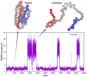
Note: Results may differ due to different random numbers generated.

---

Written by Donatas Surblys@RIKEN Theoretical molecular science laboratory
June, 2016

Updated by Yasuhiro Matsunaga@RIKEN R-CCS
May, 22, 2018

Updated by Cheng Tan@RIKEN R-CCS
Jul, 30, 2019