16.5 The enzyme reaction 1: Reaction path search
Contents
1. Introduction
In this section, QM/MM calculation is carried out using the string method [1] to search for the minimum energy path (MEP) and QSimulate-QM for the QM program. In the string method, the reaction path is discretely represented by a number of images, which propagates along the gradient component perpendicular to the path tangent. Starting from an initial path connecting the reactant and product, the images develop according to the gradient component, and converge to the MEP after iterations. In GENESIS, each image is treated with different MPI processes. Furthermore, QSimulate-QM features excellent scaling with respect to the number of computing nodes. The combination of the string method and QSimulate-QM is highly parallelizable, and thus suitable for supercomputers. For further details, see Ref. [2].
Here, we simulate a proton transfer reaction of dihyroxyacetone phosphate (DHAP) catalyzed by an enzyme, triosephosphate isomerase (TIM), which is one of the key steps in the glycolytic pathway. The reaction has been extensively studied since the early 2000 [3-8], and is a well known benchmark system [2,9]. We calculate the MEP of the following reaction:
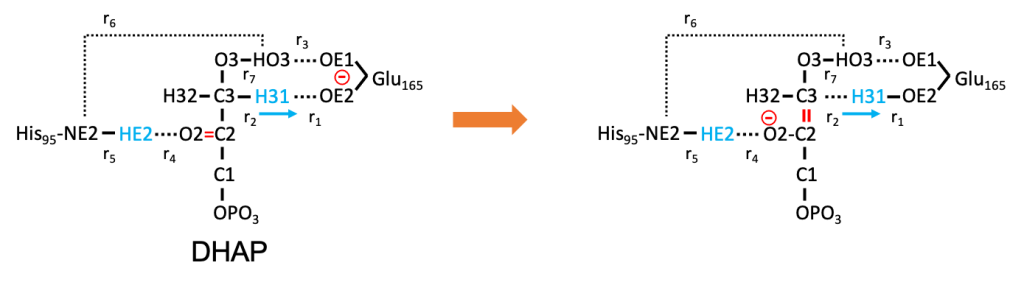
One of the proton (H31) of DHAP is transferred to Glu165 of TIM. Note that the proton transfer accompanies a charge transfer of the electron from Glu165 to O2 of DHAP (red in Fig. 1), where His95 donates a hydrogen bond. Therefore, the reaction coordinate involves not only r1 / r2 but also several intermolecular degrees of freedom (e.g., r3, r4, r6). In fact, HE2 of His95 is transferred to O2 in a later stage, though the process is beyond the scope of this tutorial.
2. System preparation
Download the tutorial file (tutorial19-16.5.zip or github), unzip it, and proceed to tutorial-16.5/1.tim. This directory contains five sub-directories.
$ unzip tutorial19-16.5.zip
$ cd tutorial-16.5/1.tim
$ ls
0.build/ 1.pre_equil/ 2.equil/ 3.min/ 4.mep/
0.build, 1.pre_equil, and 2.equil are the setup and equilibration of the system prior to QM/MM calculations. Since relevant files (pdb, psf, and rst) are retained, you can skip these steps and go directly to QM/MM calculations in 3.min. Nonetheless, let us give a brief description of these steps.
The protein structure was based on a X-ray crystal structure, 7TIM, obtained from the protein data bank.CHARMM-GUI was used to setup the system, namely, add hydrogen atoms, set the protonation states, add water molecules and ions, and so on. 0.build contains the resulting pdb and psf files.
$ ls 0.build
step2_solvator.pdb  step2_solvator.psf
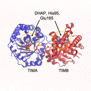
The PDB file is visualized in Fig. 2. Note that TIM is a homo-dimer (segment name TIMA and TIMB), and that the reaction site of both proteins contains the ligand.
In 1.pre_equil, the system is equilibrated in the following four MD steps.
| Step | Ensemble | Integrator | Time / ps | dt / fs |
| 3.1 | Min | – | 1,000 step | – |
| 3.2 | NVT(0.1 -> 300 K) | LEAP, Langevin | 100 | 2 |
| 3.3 | NPT (1 atm, 300K) | VVER, Bussi | 100 | 2 |
| 3.4 | NVT (300 K) | VVER, Bussi | 100 | 2 |
The positional restraints are added to the backbone (with k = 10 kcal/mol/Å2) and the sidechain, ligand, and crystal water molecules (with k = 2 kcal/mol/Å2).
$ cd 1.pre_equil
$ ls
crd_convert.inp       step3.1_minimization.inp
step3.2_heating.inp   step3.3_npt.inp     step3.4_nvt.inp
run.sh*               toppar
step3.x_*.inp are the input files of GENESIS and run.sh is a script to run the job. crd_convert.inp wraps the final trajectory, step3.4_nvt.dcd, in the simulation box. toppar contains the force field parameters. Note that the parameters of DHAP, toppar/toppar_dhap.3.str, were generated with the force field toolkit (ffTK) utility [10] of VMD.
In 2.equil, the final snapshot structure of step3.4 is first cut out to a non-periodic system using qmmm_generator. 15 Å around the TIM dimer is extracted.
Then, the system is equilibrated by NVT-MD at 300K. The positional restraints of the backbone (bb), sidechain (sc) and crystal water (cw) are gradually reduced in 8 steps, while retaining those of DHAP. In the last three steps (9 – 11), DHAP is relaxed with QM/MM-MD using DFTB3 for the QM calculations.
| Step | Potential | Time / ps | k [bb] | k [sc/cw] | k [dhap] |
| 4.1 | MM | 100 | 10 | 2 | 2 |
| 4.2 | MM | 100 | 5 | 1 | 2 |
| 4.3 | MM | 100 | 2.5 | 0.5 | 2 |
| 4.4 | MM | 100 | 1 | 0 | 2 |
| 4.5 | MM | 100 | 0.5 | 0 | 2 |
| 4.6 | MM | 100 | 0.1 | 0 | 2 |
| 4.7 | MM | 1000 | 0 | 0 | 2 |
| 4.8 | MM | 1000 | 0 | 0 | 2 |
| 4.9 | DFTB3/MM | 20 | 0 | 0 | 1 |
| 4.10 | DFTB3/MM | 20 | 0 | 0 | 0.5 |
| 4.11 | DFTB3/MM | 100 | 0 | 0 | 0 |
The files in 2.equil are as follows:
$ cd 2.equil
$ ls
qmmm_generator.inp          qsimulate.json
run.sh*                     step4.1_nvt.inp
step4.2_nvt.inp             step4.3_nvt.inp
step4.4_nvt.inp             step4.5_nvt.inp
step4.6_nvt.inp             step4.7_nvt.inp
step4.8_nvt.inp             step4.9_qmmm_nvt.inp
step4.10_qmmm_nvt.inp       step4.11_qmmm_nvt.inp
step4.11_qmmm_nvt.rst       step4_nvt_100.crd
step4_nvt_100.pdb           step4_nvt_100.psf
toppar
qmmm_generator.inp is an input file of qmmm_generator, step4.x_*.inp are the input files of GENESIS, qsimulate.json is a control file of QSimulate-QM (details are given below), and run.sh is a script to run all jobs. As a result, we obtain the files shown in red, step4_nvt_100.* (by qmmm_generator) and step4.11_qmmm_nvt.rst (by MD). These files are used in the subsequent QM/MM calculations
3. Locate the reactant and product
We first obtain the reactant and product. Proceed to 3.min,
$ cd 3.min
$ ls
min.vmd          qmmm_min2a.inp   qsimulate.json   run.sh*
qmmm_min1.inp    qmmm_min2b.inp   rst_convert.inp  toppar
qmmm_min1.inp is an input file to find the reactant,
[INPUT]
topfile = toppar/top_all36_prot.rtf, toppar/top_all36_cgenff.rtf
parfile = toppar/par_all36_prot.prm, toppar/par_all36_cgenff.prm
strfile = toppar/toppar_water_ions.str, toppar/toppar_dhap.3.str
psffile = ../2.equil/step4_nvt_100.psf     # protein structure file
pdbfile = ../2.equil/step4_nvt_100.pdb     # PDB file
reffile = ../2.equil/step4_nvt_100.pdb     # reference file
rstfile = ../2.equil/step4.11_qmmm_nvt.rst # restart file

[OUTPUT]
rstfile = qmmm_min1.rst
dcdfile = qmmm_min1.dcd

[ENERGY]
forcefield       = CHARMM
electrostatic    = CUTOFF
switchdist       = 16.0          # switch distance
cutoffdist       = 18.0          # cutoff distance
pairlistdist     = 19.5          # pair-list distance
vdw_force_switch = YES

[MINIMIZE]
method              = LBFGS      # BFGS optimizer
nsteps              = 500
eneout_period       = 1
crdout_period       = 1
rstout_period       = 1
nbupdate_period     = 1
fixatm_select_index = 2
macro               = yes   # use macro/micro-iteration scheme
nsteps_micro        = 20

[BOUNDARY]
type            = NOBC

[QMMM]
qmtyp              = qsimulate        # QSimulate-QM
qmcnt              = qsimulate.json   # control file of QSimulate-QM
workdir            = qmmm_min1
basename           = job
qmmaxtrial         = 1
qmsave_period      = 10
qmatm_select_index = 1
exclude_charge     = group

[SELECTION]
group1 = sid:DHA or (sid:TIMA and (rno:95 or rno:165) \
         and not (an:CA |an:C |an:O |an:N |an:HN |an:HA))  # QM region
group2 = not (sid:DHA or sid:DHA around_res:6.0) # fixed atoms during minimization
The important options are highlighted in red with comments in blue. Note that:
- [INPUT]: The files in
2.equilare used to restart the job. - [ENERGY]: The switch and cutoff distances are longer than usual.
- [MINIMIZE]: The L-BFGS algorithm is specified with macro/micro-iteration scheme.
- [QMMM]: QSimulate-QM is specified for a QM program.
qmexeis not needed, because GENESIS and QSimulate-QM are linked through dynamic libraries. - [SELECTION]: group1 is the QM region (DHAP and sidechain of His95 and Glu165), and group2 specifies fixed MM atoms.
qsimulate.json is a control file of QSimulate-QM, which specifies the level of DFT calculations,
{ "bagel" : [

{
  "title" : "molecule",
  "basis" : "aug-cc-pvdz",            .... (1)
  "df_basis" : "cc-pvdz-jkfit",       .... (1)
  "basis_link" : "cc-pvdz",           .... (2)
  "df_basis_link" : "cc-pvdz-jkfit"   .... (2)
},

{
  "title" : "force",
  "method" : [ {
    "title" : "ks",
    "charge" : -3,                    .... (3)
    "xc_func" : "b3lyp",              .... (4)
    "dispersion" : true,              .... (4)
    "population" : true               .... (5)
  } ]
}

]}
- The orbital basis sets and the density fitting basis sets are specified by “basis” and “df_basis”, respectively. Here, we use Dunning’s aug-cc-pVDZ basis sets.
- Similarly, “basis_link” and “df_basis_link” specify the basis sets of link hydrogen atoms. It is better not to add diffuse functions to the link hydrogen, because they often cause overpolarization due to nearby MM charges and make the calculation unstable.
- Total charge of the QM region. -2 of DHAP and -1 of Glu165.
- B3LYP functional with D3(BJ) dispersion corrections
- Calculates the intrinsic atomic-orbital (IAO) charges. The charge is used in macro/micro-iteration scheme.
qmmm_min2a.inp and qmmm_min2b.inp are input files to find the product. qmmm_min2a.inp is similar to qmmm_min1.inp except for the following restraints,
[MINIMIZE]
method              = LBFGS
nsteps              = 50   # number of steps
...


[SELECTION]
...
group3     = atomno:2560 # OE2 of Glu165
group4     = atomno:7588 # H31 of DHAP
group5     = atomno:7585 # C3  of DHAP

[RESTRAINTS]
nfunctions    = 2
function1     = DIST     # create OE2-H31
constant1     = 100.0
reference1    = 1.0
select_index1 = 3 4
function2     = DIST     # dissociate C3 ... H31
constant2     = 100.0
reference2    = 2.5
select_index2 = 4 5
These strong distant restraints moves the proton (H31) from DHAP to Glu165. The minimization is carried out only for a small number of steps (= 50), so it does not converge. Yet, 50-iteration is sufficient to move the proton close to Glu165, and to make the whole structure close to the product. Then, qmmm_min2b.inp restarts a regular minimization without restraints and yields a fully optimized product state.
run.sh is a script to run the job.
#!/bin/bash

export LD_LIBRARY_PATH=/path/to/qsimulate/lib:$LD_LIBRARY_PATH  ... (1)
export PATH=$PATH:/path/to/genesis/bin   ... (2)

export OMP_NUM_THREADS=4
export BAGEL_NUM_THREADS=${OMP_NUM_THREADS}
export MKL_NUM_THREADS=${OMP_NUM_THREADS}
export I_MPI_PERHOST=4
export I_MPI_DEBUG=5

mpiexec.hydra -n 8 atdyn qmmm_min1.inp  >& qmmm_min1.out ... (3)
sed "s/MIN/min1/" rst_convert.inp  > aa
rst_convert aa > /dev/null                ... (4)
rm aa

mpiexec.hydra -n 8 atdyn qmmm_min2a.inp >& qmmm_min2a.out ... (3)
mpiexec.hydra -n 8 atdyn qmmm_min2b.inp >& qmmm_min2b.out ... (3)
sed "s/MIN/min2b/" rst_convert.inp  > aa
rst_convert aa > /dev/null                ... (4)
rm aa

exit 0
- Set the LD_LIBRARY_PATH to where the dynamic libraries of QSimulate-QM are installed.
- Set the PATH to where GENESIS is installed.
- GENESIS jobs for min1, min2a, and min2b.
- rst_convert converts rst file to pdb file
In the script, OMP_NUM_THREADS and I_MPI_PERHOST control the number of thread per MPI process and the number of MPI processes per node, respectively. The number of MPI processes is specified after “-n” of the mpiexec.hydra command. Thus, assuming that two 16-core nodes are available, the above script uses 4 thread x 8 MPI processes in total, allocating 4 thread x 4 MPI processes per node. Adjust the numbers in blue so as to fit to your computational resources.
Now, run the job,
$ ./run.sh
After the job ends, check if the minimization job converged or not. If the message, “RMSG and MAXG becomes sufficiently small”, is printed, the minimization has successfully converged.
$ grep ">>>>>" qmmm_min1.out qmmm_min2b.out
qmmm_min1.out: >>>>> STOP: RMSG and MAXG becomes sufficiently small
qmmm_min2b.out: >>>>> STOP: RMSG and MAXG becomes sufficiently small
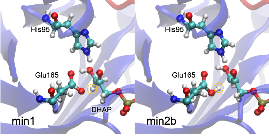
The structure of the reactant and product can be visualized using VMD,
$ vmd -e min.vmd
This command gives Fig. 4, which shows that the proton of DHAP is transferred to Glu165.
4. MEP search
We now calculate the MEP that connects the reactant and product obtained in the previous subsection. Go to 4.mep, and you will find three sub-directories.
$ cd 4.mep
$ ls
0.initial16/ 1.string16/  2.analysis/
4.1. The initial path
The string method requires an initial path as an input. Thus, we first generate a path that connects the reactant and product obtained in the previous subsection. Proceed to 0.initial16,
$ cd 0.initial16
$ ls
initial.vmd   mk_initial_path.f90   mk_initial_path.sh
mk_initial_path.f90 is a fortran program to generate the path. Given two pdb files and the number of image, the program yields a series of structures that linearly connects the two pdb structures in terms of Cartesian coordinates. mk_initial_path.sh is a script to compile and execute the program,
$ cat mk_initial_path.sh
gfortran mk_initial_path.f90 -o mk_initial_path
./mk_initial_path ../../3.min/qmmm_min1.pdb ../../3.min/qmmm_min2b.pdb 16
The first line compiles the code using gfortran. Any other fortran compiler should be OK. In that case, replace gfortran with an appropriate command. The second line executes the program. The first and the second arguments are pdb files of the two end-point, i.e., the reactant and product, respectively, and the third arguement is the number of images.
Now, run the script,
$ ./mk_initial_path.sh
$ ls
initial.vmd          initial12.pdb        initial16.pdb
initial1.pdb         initial13.pdb        initial2.pdb
...
initial*.pdb is the initial reation path. You can visualize the inital path using initial.vmd.
$ vmd -e initial.vmd
4.2. The string calculation
We now carry out the string calculation. Proceed to 1.string16,
$ cd ../1.string16
$ ls
qmmm_mep.inp    qsimulate.json    run.sh*    toppar
qmmm_mep.inp is an input file. We show in the following the options specific to the string calculation:
[INPUT]
...
pdbfile = ../0.initial16/initial{}.pdb   # Initial path

[OUTPUT]
dcdfile = mep_{}.dcd
logfile = mep_{}.log
rstfile = mep_{}.rst
rpathfile  = mep_{}.rpath

[ENERGY]
...

[MINIMIZE]
method              = LBFGS
nsteps              = 200
eneout_period       = 2     # energy output to log file
nbupdate_period     = 1
fixatm_select_index = 2
macro               = yes   # use macro/micro-iteration scheme
nsteps_micro        = 20

[RPATH]
rpathmode           = MEP     # MEP search
method              = STRING  # use the string method
delta               = 0.0005  # stepsize of the propagation
ncycle              = 200     # max number of cycle
nreplica            = 16      # number of replicas
eneout_period       = 1       # energy output period
crdout_period       = 1       # coordinates output period
rstout_period       = 1       # restart output period
fix_terminal        = no      # fix the end-points
massWeightCoord     = no      # mass-weight coorindates
mepatm_select_index = 1       # target atoms of MEP search

[BOUNDARY]
...

[QMMM]
...

[SELECTION]
...
- [INPUT] and [OUTPUT]: The initial path is specified by
pdbfile. The curvy braket ({}) is replaced by replica ID at runtime. - [RPATH]:
rpathmode = MEPinvokes the MEP search.method = stringinvokes the string method.nreplica = 16is the number of images. This must be consistent with the number of initial images.mepatm_select_indexspecifies MEP atoms. The MEP is searched in terms of Cartesian coordinates of these atoms. All QM atoms must be included in the MEP atoms. In addition, MM atoms can be included in MEP atoms, although it is rarely needed to do so. MEP atoms are taken to be the same as QM atoms (= group1) in this case.
- [MINIMIZE]: The MM atoms not included in the MEP atoms are energy minimized with the MEP atoms fixed. Therefore, [MINIMIZE] section is always needed in the MEP search. It is strongly recommended to use
macro=yes. In this case, the minimization is performed with the QM atoms (= MEP atoms) replaced by QM charges like in the micro-iteration scheme. On the other hand, ifmacro=no, QM calculations are required every step of the MM minimization, so that the cost increases enormously.
qsimulate.json is exactly the same as before. run.sh is also similar except that the number of MPI processes is now 128. We assign 8 MPI processes for each replica, so that 8 MPI x 16 replicas = 128 MPI in total.
#!/bin/bash
#
export LD_LIBRARY_PATH=/path/to/qsimulate/lib:$LD_LIBRARY_PATH
export PATH=$PATH:/path/to/genesis/bin

export OMP_NUM_THREADS=4
export BAGEL_NUM_THREADS=${OMP_NUM_THREADS}
export MKL_NUM_THREADS=${OMP_NUM_THREADS}
export I_MPI_PERHOST=4
export I_MPI_DEBUG=5

mpiexec.hydra -n 128 atdyn qmmm_mep.inp >& qmmm_mep.out

exit 0
The number of MPI processes must be multiples or divisors of the number of replicas. In this example, we have 16 replicas, so 160 MPI is OK but 150 MPI is not. Also, 2, 4, 8 MPI are OK but 3, 5, 6, 7 is not. Note that 1 MPI process is assigned to each replica when it is set to the divisors. Thus, we need to pay careful attention when setting the number of replicas. For example, 16 replicas may be more flexible than 17 replicas.
Now, run the script,
$ ./run.sh
If the job starts successfully, you will see the first iteration of the MEP search in the output like this,
Iter.     1

         Path Length   Energy (kcal/mol)    Relative E.   Energy Conv.
---------------------------------------------------------------------------
Image   1     0.0000       -1006333.1906         0.0000        -0.0335
Image   2     0.1564       -1006332.2065         0.9841        -0.0444
Image   3     0.3136       -1006329.3782         3.8124        -0.0824

...

Image  15     2.1932       -1006319.1649        14.0257        -0.5713
Image  16     2.3496       -1006321.4105        11.7801        -0.6897
---------------------------------------------------------------------------
   Energy Conv. (Max) =          -0.68972754
   Path length: current value / variation =      2.34960315 /     2.34960315
The cycle is iterated until the energy and the path length converge within a threshold value. When the convergence is achieved, you will see a message, “Convergence achieved”.
Iter.    93

         Path Length   Energy (kcal/mol)    Relative E.   Energy Conv.
---------------------------------------------------------------------------
Image   1     0.0000       -1006333.2068         0.0000         0.0000
Image   2     0.2014       -1006333.0839         0.1230        -0.0005
Image   3     0.4027       -1006332.6858         0.5211        -0.0020
Image   4     0.6041       -1006331.9645         1.2423        -0.0024
Image   5     0.8055       -1006330.8851         2.3217        -0.0028
Image   6     1.0068       -1006329.5409         3.6659        -0.0026
Image   7     1.2082       -1006327.9563         5.2505        -0.0020
Image   8     1.4096       -1006326.2708         6.9361        -0.0018
Image   9     1.6111       -1006324.5610         8.6459        -0.0012
Image  10     1.8126       -1006322.9791        10.2277        -0.0030
Image  11     2.0134       -1006320.9835        12.2233        -0.0037
Image  12     2.2148       -1006317.7300        15.4768        -0.0059
Image  13     2.4176       -1006318.6608        14.5460        -0.0099
Image  14     2.6161       -1006320.6838        12.5230        -0.0041
Image  15     2.8168       -1006321.3417        11.8652        -0.0011
Image  16     3.0180       -1006321.5579        11.6489        -0.0003
---------------------------------------------------------------------------
   Energy Conv. (Max) =          -0.00988236
   Path length: current value / variation =      3.01804347 /     0.00413513
Convergence achieved in 93 iterations
4.3. Analysis
After the MEP search is finished, we now analyze the results. Go to 2.analysis,
$ cd ../2.analysis
$ ls
analysis.sh       mep.vmd           rpath_r_img.gpi
data/             rpath_OHCH.gpi    rst_convert.inp
makedat.f90       rpath_ene.gpi     trj_analysis.inp
analysis.sh is a script to run the analysis,
#!/bin/bash

export PATH=${PATH}:/path/to/genesis/bin     ... (1)

NIMG=$(ls -l ../0.initial16/*pdb |wc -l)
NAME=mep

rm ${NAME}_*dis
rm ${NAME}_*.pdb
for i in `seq 1 ${NIMG}`; do
  echo ${i}

  # get r1 - r7
  sed "s/NAME/${NAME}/g" trj_analysis.inp  >& aa
  sed "s/NUM/${i}/g" aa  >& trj_analysis${i}.inp
  trj_analysis trj_analysis${i}.inp >& trj_analysis${i}.out   ... (2)
  rm trj_analysis${i}.inp trj_analysis${i}.out aa

  # get pdbfiles
  sed "s/NAME/${NAME}/g" rst_convert.inp  >& aa
  sed "s/NUM/${i}/g" aa  >& rst_convert${i}.inp
  rst_convert rst_convert${i}.inp >& rst_convert${i}.out      ... (3)
  rm rst_convert${i}.inp rst_convert${i}.out aa
done

# get dat files
gfortran makedat.f90 -o makedat                   ... (4)
./makedat -output ../1.string16/qmmm_mep.out \
          -disout mep_{}.dis -interval 10    \
          -basename rpath_ >& makedat.out         ... (4)
- Set the PATH to where GENESIS is installed.
- Calculates r1 – r7 of each replica and prints them to mep_{}.dis
- Converts rst file to pdb file for each replica
- makedat is a fortran program that reads the energy (from GENESIS output) and the distance (from *.dis) and prints the information to rpath_xx.dat, where xx is the count of iteration.
Now run the analysis,
$ ./analysis.sh
1
2
...
16
The coordinates of the final path (=MEP) are given in mep_*.pdb. They can be visualized by VMD,
$ vmd -e mep.vmd
The information of the path in each iteration is given in rpath_*.dat.
$ ls rpath*_dat
rpath_0.dat   rpath_21.dat  rpath_51.dat  rpath_81.dat
rpath_1.dat   rpath_31.dat  rpath_61.dat  rpath_91.dat
rpath_11.dat  rpath_41.dat  rpath_71.dat  rpath_93.dat
The interval of printing is set by “-interval” option in makedat (see the last line of analysis.sh). In the above example, rpath_93.dat is the converged MEP. Note that the count of iteration may or may not be 93 in your calculation, though it is expected to be around 90 – 100. The rpath_*.dat files are logged in the following format,
$ cat rpath_93.dat
   1   0.0000   0.0000    2.530    1.098    1.762    1.869    1.023    2.777    0.994
   2   0.2014   0.1230    2.449    1.097    1.782    1.862    1.023    2.765    0.993
...
The first column is the ID of images. The second and the third columns are the pathlength and the relative energy (in kcal/mol), respectively. The fourth to the 10th columns are the atomic distances, r1, r2, … , r7.
rpath*gpi are gnuplot scripts to plot the results. rpath_ene.gpi and rpath_OHCH.gpi plots the variation of the energy profile and the geometry, respectively. The script is executed by,
$ gnuplot rpath_ene.gpi
$ gnuplot rpath_OHCH.gpi
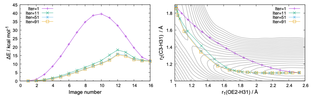
The command creates pdf files shown in Fig. 5. It is clear that the MEP is nicely converged both in terms of energy and geometry. rpath_r_img.gpi plots the variation of r1 – r7 as a function of the image ID,
$ gnuplot rpath_r_img.gpi
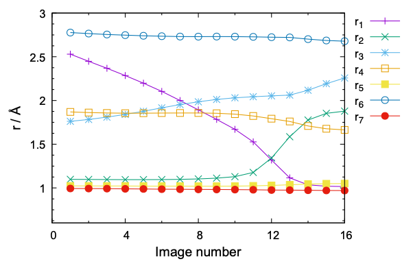
The plot shown in Fig. 6 indicates that not only r1/r2 but also r3 (HO3 … OE1) and r4 (HE2 … O2) are affected by the proton transfer reaction.
5. Concluding remarks
We have demonstrated the MEP search of the first proton transfer reaction from DHAP to Glu165 of TIM. The protocol consists of 4 steps:
- Setup and equilibrate the system (
0.build,1.pre_equil) - Setup a cluster system and carry out equilibration MDs (
2.equil) - Locate the reactant and product structures by minimization (
3.min) - Search the MEP using the string method (
4.mep)
This scheme is applicable to other reactive systems as well. Interested readers are encouraged to try proton transfer reactions of TIM in the later stage [2]. Another example is available for chorismate mutase in 2.cm.
We have also demonstrated the usage of QSimulate-QM. Here, the QM calculations have been performed at the B3LYP-D3/aug-cc-pVDZ level. Various electronic structure methods are available, for example, DFTB3, pure and hybrid DFT, RI-MP2, multireference methods (CASPT2), and so on. Refer to the manual of QSimulate-QM for how to set the options in qsimulate.json.
The caveat of the present scheme is that MEP is a static analysis, lacking in dynamical and entropic effects. In the next subsection, we perform replica-exchange umbrella sampling (REUS) simulations using the MEP as a collective variable and calculate the free-energy profile along the MEP.
References
- W. E, W. Ren, and E. Vanden-Eijnden, J. Chem. Phys. 126, 164103 (2007).
- K. Yagi, S. Ito, and Y. Sugita, J. Phys. Chem. B 125, 4701 – 4713 (2021).
- Q. Cui and M. Karplus, J. Am. Chem. Soc. 123, 2284-2290 (2001).
- Q. Cui and M. Karplus, J. Am. Chem. Soc. 124, 3093–3124 (2002).
- Q. Cui and M. Karplus, J. Phys. Chem. B 106, 1768-1798 (2002).
- C. Lennartz, A. Schäfer, F. Terstegen, and W. Thiel, J. Phys. Chem. B 106, 1758-1767 (2002).
- Y. Zhang, H. Liu, and W. Yang, J. Chem. Phys. 112, 3483 (2000).
- H. Hu, Z. Lu, and W. Yang, J. Chem. Theory Comput. 3, 390-406 (2007).
- J. I. Mendieta-Moreno, R. C. Walker, J. P. Lewis, P. Gómez-Puertas, J. Mendieta, and J. Ortega, J. Chem. Theory Comput. 10, 2185-2193 (2014).
- C. G. Mayne, J. Saam, K. Schulten, E. Tajkhorshid, J. C. Gumbart, J. Comput. Chem. 34, 2757-2770 (2013).
Written by Kiyoshi Yagi@RIKEN Theoretical molecular science laboratory
April., 3, 2022