13.1 Conformational sampling of ala-dipeptide in water using Gaussian accelerated molecular dynamics
Contents
The Gaussian accelerated Molecular Dynamics (GaMD) method [1,2] accelerates the conformational sampling of biomolecules by adding a harmonic boost potential to smooth the potential energy of a biological system:
\( \displaystyle U'(x) = U(x)+\Delta U^{\text{GaMD}}\left(U(x)\right),\\ \displaystyle \Delta U^{\text{GaMD}}\left(U(x)\right) = \begin{cases}\frac{1}{2}k\left\{E-U(x)\right\}^2 & (U(x) < E)\\ 0 & (U(x)\ge E),\end{cases}\)
where \(x\) is the configuration of the system, \(U\) is the potential energy, \(\Delta U^{\text{GaMD}}\) is the boost potential of GaMD, the prime represents the value biased by GaMD boosting, \(k\) is a harmonic force constant, and \(E\) is the threshold of GaMD. As shown in Figure 1, we can see that the boost potential is added to the original potential surface, which lowers the energy barrier between basins.
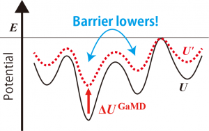
Figure 1. Scheme of GaMD boosting.
GaMD does not require predefined reaction coordinates, which is a significant advantage because expert knowledge of the biomolecular systems of interest is essential for the definition of reaction coordinates. The use of the harmonic boost potential allows us to recover the unbiased free-energy changes through cumulant expansion to the second order, which resolves the practical reweighting problems in the original accelerated MD [3]. Here, we demonstrate a GaMD simulation by employing the alanine dipeptide as an example.
Note: GPU acceleration is available in GaMD simulations. If you have GPUs, we strongly recommend you to use GPUs. Please see here for GENESIS installation to GPU machines.
Preparation
First of all, let’s download the tutorial file (tutorial-13.1.tar.gz ). This tutorial consists of six steps: 1) system setup, 2) minimization, heating, and equilibration, 3) determination of initial parameters of GaMD by a short simulation, 4) determination of GaMD parameters with updating, 5) production run of GaMD, and 6) trajectory analysis. Control files for GENESIS are already included in the download file.
# Download the tutorial file
$ cd /home/user/GENESIS/Tutorials
$ mv ~/Downloads/tutorial-13.1.tar.gz ./
$ tar -xzvf tutorial-13.1.tar.gz
$ cd tutorial-13.1
$ ls
1_setup  2_equil  3_gamd_init  4_gamd_update  5_gamd_prod  6_anal
1. Setup
In this tutorial, we perform GaMD of alanine dipeptide in water. In the following commands, we build the system using tLeap which is included in AmberTools. If you do not have AmberTools, please download it from here. We obtain ionize.pdb, ionize.inpcrd, and ionize.prmtop as the input files for GENESIS.
# Change directory for the system setup
$ cd 1_setup
$ ls
alad.pdb  run.sh

# Make inpcrd and prmtop files using tLeap
$ run.sh
$ ls
alad.pdb  ionize.inpcrd  ionize.pdb  ionize.prmtop  leap.log  run.sh

# View the initial structure
$ vmd ionize.prmtop ionize.pdb
2. Minimization, heating, and equilibration
We carry out energy minimization, heating, and equilibration of the system. Please refer to Tutorial 3.2, for details about input options.
# Change directory for equilibration
$ cd ../2_equil
$ ls
run.sh  run1.inp  run2.inp  run3.inp
First, we perform a 5000-step minimization of the system to remove non-physical steric clashes. run1.inp is a control file for the minimization.
# Perform minimization
$ /home/user/GENESIS/bin/spdyn -np 8 run1.inp > run1.out
Next, we heat up the system from 0.1 K to 300 K during a 100-picosecond molecular dynamics simulation. run2.inp is a control file for heating.
# Perform heating
$ /home/user/GENESIS/bin/spdyn -np 8 run2.inp > run2.out
In the equilibration run, we carry out a 100-ps MD simulation at 300 K and 1 atm using the Bussi thermostat and barostat. run3.inp is a control file for equilibration. The equations of motion are integrated with the velocity Verlet algorithm with the time step of 2 fs, where the SHAKE algorithm is used for bond constraint.
# Perform equilibration
$ /home/user/GENESIS/bin/spdyn -np 8 run3.inp > run3.out

# View the trajectory using VMD
$ vmd ../1_setup/ionize.prmtop -dcd run3.dcd
3. Determination of initial parameters of GaMD by a short simulation
In this tutorial, we use the dual boost scheme of GaMD, in which not only the dihedral potential but also the total potential of the system are independently boosted by harmonic potentials. We first determine initial parameters for GaMD dual boosting (i.e., pot_max, pot_min, pot_ave, pot_dev, dih_max, dih_min, dih_ave, dih_dev). The harmonic constant \(k\) and the threshold \(E\) in the above equation are determined from these parameters. Please refer to GENESIS manual or the original papers of GaMD [1,2] for more detail. To obtain the initial guess of the boosting potential, we perform a short MD simulation without GaMD boosting. The following command executes the simulation:
$ cd ../3_gamd_init
$ /home/user/GENESIS/bin/spdyn -np 8 run.inp > run.out
The following shows the most important parts in run.inp. In [GAMD] section, we set the keyword related to GaMD. GaMD is turned on by gamd = yes. boost = no means that GaMD boosts are not applied but GaMD parameters are updated from the trajectory. In this example, we use the dual boost scheme and set the threshold of GaMD to the lower bound, which are specified by boost_type = DUAL and thresh_type = LOWER, respectively. sigma0_pot and sigma0_dih are the upper limit of the standard deviation of the total potential boost and that of the dihedral potential boost, respectively. These parameters are required for accurate reweighting. We here set these values to 6 kcal/mol. update_period in [GaMD] section is an update frequency of GaMD parameters. GaMD parameters are updated every update_period steps. At the same time, the updated parameters are output to gamdfile in [OUTPUT]. For the initial determination of parameters, update_period should be set to the same as nsteps in [DYNAMICS].
[OUTPUT]
dcdfile  = run.dcd
rstfile  = run.rst
gamdfile = run.gamd

[GAMD]
gamd          = yes
boost         = no
boost_type    = DUAL
thresh_type   = LOWER
sigma0_pot    = 6.0
sigma0_dih    = 6.0
update_period = 500000
The example of GaMD output file (gamdfile) is shown below.
            STEP         POT_MAX         POT_MIN         POT_AVE         POT_DEV          POT_TH          POT_KC         POT_KC0         DIH_MAX         DIH_MIN         DIH_AVE         DIH_DEV          DIH_TH          DIH_KC         DIH_KC0
 --------------- --------------- --------------- --------------- ---------------
          500000     -20927.9358     -21470.9234     -21170.3356         66.0818     -20927.9358          0.0003          0.1640         18.8888          8.4258         11.0364          1.0713         18.8888          0.0956          1.0000
4. Determination of GaMD parameters with updating
In this step, we determine GaMD parameters by updating them at each update_period period. The following command executes the simulation:
$ cd ../4_gamd_update
$ /home/user/GENESIS/bin/spdyn -np 8 run.inp > run.out
The most important parts in run.inp are shown below. To turn on GaMD boosting, we set boost = yes in this step. The values of pot_max, pot_min, pot_ave, pot_dev, dih_max, dih_min, dih_ave, and dih_dev are initially set to the parameters determined in the previous step (i.e., the values in the last line in gamdfile). We here specify the update frequency of GaMD parameters by update_period = 500. From the energy trajectory of 500 steps, the maximum, minimum, average, and standard deviation of the energy are calculated, and then the corresponding GaMD parameters are updated. The updated parameters are output to gamdfile in [OUTPUT] every update_period = 500 period.
[OUTPUT]
dcdfile  = run.dcd
rstfile  = run.rst
gamdfile = run.gamd

[GAMD]
gamd          = yes
boost         = yes
boost_type    = DUAL
thresh_type   = LOWER
sigma0_pot    = 6.0
sigma0_dih    = 6.0
update_period = 500
pot_max       = -20927.9358
pot_min       = -21470.9234
pot_ave       = -21170.3356
pot_dev       = 66.0818
dih_max       = 18.8888
dih_min       = 8.4258
dih_ave       = 11.0364
dih_dev       = 1.0713
The example of GaMD output file is shown below. Parameter updating should be continued until the parameters converge. The parameters in the last line of gamdfile are used for the production run.
            STEP         POT_MAX         POT_MIN         POT_AVE         POT_DEV          POT_TH          POT_KC         POT_KC0         DIH_MAX         DIH_MIN         DIH_AVE         DIH_DEV          DIH_TH          DIH_KC         DIH_KC0
 --------------- --------------- --------------- --------------- ---------------
             500     -20927.9358     -21470.9234     -21023.5243         31.8438     -20927.9358          0.0004          0.2287         18.8888          8.4258         11.5085          1.0981         18.8888          0.0956          1.0000


            1000     -20927.9358     -21470.9234     -21019.7042         30.3392     -20927.9358          0.0004          0.2380         18.8888          8.4258         12.0291          1.4921         18.8888          0.0956          1.0000
…
…
…
         2499500     -20630.7328     -21470.9234     -20854.8429         44.3726     -20630.7328          0.0002          0.1844         28.6641          8.4258         13.6859          1.8830         28.6641          0.0494          1.0000


         2500000     -20630.7328     -21470.9234     -20854.8335         44.3752     -20630.7328          0.0002          0.1844         28.6641          8.4258         13.6857          1.8830         28.6641          0.0494          1.0000
5. Production run of GaMD
In this step, we perform the production run of GaMD. The following command executes the simulation:
$ cd ../5_gamd_prod
$ /home/user/GENESIS/bin/spdyn -np 8 run.inp > run.out
The most important parts in run.inp are shown below. The values of pot_max, pot_min, pot_ave, pot_dev, dih_max, dih_min, dih_ave, and dih_dev are set to the parameters obtained in the previous step. Since GaMD parameters should not be changed in production MDs, we specify update_period = 0. We notice that the frequency of output should be high, i.e., eneout_period = 50 and crdout_period = 50 in order to reweight the GaMD trajectory accurately.
[OUTPUT]
dcdfile  = run.dcd
rstfile  = run.rst
gamdfile = run.gamd

[GAMD]
gamd          = yes
boost         = yes
boost_type    = DUAL
thresh_type   = LOWER
sigma0_pot    = 6.0
sigma0_dih    = 6.0
update_period = 0
pot_max       = -20630.7328
pot_min       = -21470.9234
pot_ave       = -20854.8335
pot_dev       = 44.3752
dih_max       = 28.6641
dih_min       = 8.4258
dih_ave       = 13.6857
dih_dev       = 1.8830
6. Analysis
6.1 Calculation of dihedral angles of alanine dipeptide
We calculate the free-energy landscape in a 2-dimensional dihedral angle space. First, we extract dihedral angles from the trajectory. The following command calculates the dihedral angles of the alanine dipeptide:
$ cd ../6_anal/1_calc_cv
$ ./run.sh
The content of run.sh is shown below. This script calculates Φ (torsion 1) and Ψ (torsion 2) dihedral angles (shown in Figure 2) of alanine dipeptide from run.dcd which is obtained by the GaMD simulation. The values of the dihedrals are output to “cv.dat”.
#!/bin/bash

rm cv.dat

cat << EOF > cv.inp
[INPUT]
prmtopfile = ../../1_setup/ionize.prmtop
reffile    = ../../1_setup/ionize.pdb

[OUTPUT]
torfile = cv.dat

[TRAJECTORY]
trjfile1      = ../../5_gamd_prod/run.dcd
md_step1      = 1000000                      # number of MD steps
mdout_period1 = 1                            # MD output period
ana_period1   = 1                            # analysis period
repeat1       = 1
trj_format    = DCD                          # (PDB/DCD)
trj_type      = COOR+BOX                     # (COOR/COOR+BOX)

[OPTION]
check_only = NO
torsion1   = 1:ACE:C 2:ALA:N  2:ALA:CA 2:ALA:C       # PHI angle
torsion2   = 2:ALA:N 2:ALA:CA 2:ALA:C  3:NME:N       # PSI angle
EOF

trj_analysis cv.inp

rm cv.inp
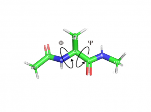
Figure 2. Dihedral angles of alanine dipeptide.
6.2 Reweighting
The distribution of dihedral angles obtained in the previous step is not yet reweighted, that is, the free energy landscape of the dihedrals is still imposed by the GaMD boost potentials. We here reweight the free-energy landscape. The unbiased probability distribution of the CV of interest can be obtained by following equations:
\( \displaystyle p(\xi) = \frac{\int \delta (\xi-\xi(x))\exp [-\beta U(x)] dx}{\int \exp [-\beta U(x)] dx} \\ \displaystyle =\frac{\int \delta (\xi-\xi(x))\exp [\beta \Delta U^{\text{GaMD}}(x)] \exp [-\beta U'(x)] dx}{\int \delta (\xi-\xi(x)) \exp [-\beta U'(x)] dx} \frac{\int \delta (\xi-\xi(x))\exp [-\beta U'(x)] dx}{\int \exp [-\beta U'(x)] dx} \\ \displaystyle \frac{\int \exp [-\beta U'(x)] dx}{\int \exp [\beta \Delta U^{\text{GaMD}}(x)] \exp [-\beta U'(x)] dx} \\ \displaystyle = \left<\exp[\beta \Delta U^{\text{GaMD}}]\right>’_{\xi} \frac{p'(\xi)}{\left<\exp[\beta \Delta U^{\text{GaMD}}]\right>’},\)
where \(\xi\) is the CV. First, we extract the GaMD boost potentials \(\Delta U^{\text{GaMD}}\) from the GENESIS log file.
$ cd ../2_reweight_gamd
$ grep "^INFO" ../../5_gamd_prod/run.out > out.dat
The example of out.dat is shown below. The values in 17th and 18th columns correspond to the boost potentials of the total potential and dihedral energies, respectively.
INFO:       STEP            TIME       TOTAL_ENE   POTENTIAL_ENE     KINETIC_ENE            RMSG            BOND           ANGLE        DIHEDRAL        IMPROPER         VDWAALS   DISP-CORR_ENE           ELECT     TEMPERATURE          VOLUME  POTENTIAL_GAMD   DIHEDRAL_GAMD
INFO:         50          0.1000     -16913.7735     -21081.7653       4151.8457         13.0088          3.0848         10.7171         11.3267          0.2241       3287.3677       -180.4632     -24214.0226        310.7003      67975.4663          8.7200          7.4261
INFO:        100          0.2000     -16910.0513     -21044.4349       4122.8594         13.1644          5.5444          8.3032         14.7615          0.3908       3308.6533       -180.4632     -24201.6250        308.5311      67975.4663          6.7491          4.7751
…
…
…
From out.dat and cv.dat, we can obtain the reweighted free-energy landscape according to above equations. However, the convergence of \( \left<\exp[\beta \Delta U^{\text{GaMD}}]\right>’_{\xi} \) is very slow, which causes the large statistical error. To reduce the statistical error, the cumulant expansion to the second order has been employed for GaMD simulations [4]. We do the cumulant expansion by the following commands.
./gamd_reweight_2d.py -t 300.0 -c 10 -n 1000000 --Xmin -180 --Xmax 180 --Xdel 10 --Ymin -180 --Ymax 180 --Ydel 10 --cv_file ../1_calc_cv/cv.dat --out_file out.dat --Xcyclic --Ycyclic
./plot_pmf_2d.py
gamd_reweight_2d.py reweights the free-energy landscape. The absolute temperature, the number of samples, the minimum value of the CV, the maximum value of the CV, the grid size of the bin for the CV are assigned by “-t”, “-n”, “–Xmin”, “–Xmax”, “–Xdel”, respectively. “-c” represents the cutoff of the number of samples in each bin. If the number of samples in a certain bin is below 10, the probability (or free energy) in the bin is omitted. “–Xcyclic” represents the periodicity of the CV. This script outputs the free energies in each bin “pmf.dat” and grid points of the CVs “xi.dat” and “yi.dat”. plot_pmf_2d.py draws the two-dimensional free-energy landscape using “pmf.dat”, “xi.dat”, and “yi.dat”.
The free-energy landscape reconstructed from the obtained dihedral angles and GaMD boost potentials is shown in Figure 3. The population of each conformational state is consistent with the results of the earlier studies in the literature.
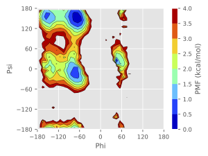
Figure 3. The reweighted free-energy landscape of two dihedral angles of alanine dipeptide.
You can obtain the free-energy landscape without reweighting according to the following commands.
./gamd_reweight_2d.py -t 300.0 -c 10 -n 1000000 --Xmin -180 --Xmax 180 --Xdel 10 --Ymin -180 --Ymax 180 --Ydel 10 --cv_file ../1_calc_cv/cv.dat --out_file out.dat --Xcyclic --Ycyclic --noreweight
./plot_pmf_2d.py
The unreweighted free-energy landscape constructed from the obtained dihedral angles is shown in Figure 4. Due to the GaMD biases, the populations of the αR and C7ex conformations are overestimated, while the β/C5 conformation is underestimated. We can confirm that these overestimation and underestimations are modified in the above reweighting.
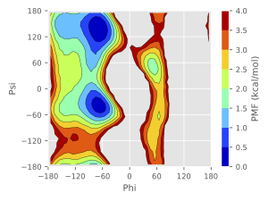
Figure 4. The unreweighted free-energy landscape of two dihedral angles of alanine dipeptide.
References
- Y. Miao, V. A. Feher, and J. A. McCammon. Gaussian Accelerated Molecular Dynamics: Unconstrained Enhanced Sampling and Free Energy Calculation. J. Chem. Theory Comput., 11, 3584–3595 (2015).
- Y. T. Pang, Y. Miao, Y. Wang, and J. A. McCammon. Gaussian Accelerated Molecular Dynamics in NAMD. J. Chem. Theory Comput., 13, 9–19 (2017).
- D. Hamelberg, J. Mongan, and J. A. McCammon. Accelerated Molecular Dynamics: A Promising and Efficient Simulation Method for Biomolecules. J. Chem. Phys., 120, 11919–11929 (2004).
- Y. Miao, W. Sinko, L. Pierce, D. Bucher, R. C. Walker, and J. A. McCammon. Improved Reweighting of Accelerated Molecular Dynamics Simulations for Free Energy Calculation. J. Chem. Theory Comput., 10, 2677–2689 (2014).
Written by Hiraku Oshima@RIKEN BDR
September, 2, 2019