1.2 Let’s take a quick look at the source code of GENESIS
Contents
Take a look at the source directory
In this tutorial, we briefly explain the source code of GENESIS. We expect that you have already learned basic theories of MD simulations [1,2,3]. Even if you are an experimental scientist, we recommend you to take a look at the source code of GENESIS for a better understanding of the MD algorithm. GENESIS is written mainly in Fortran90, which is a traditional language but still widely used in the computational science due to its simplicity. Let’s go to the directory where the source code of the MD program atdyn is contained. In this directory, you will find many files with the filename extensions .fpp, .f90, .o, and .mod. Of these, fpp file is the original source code, while the other files were generated after the compilation. Therefore, we will mainly focus on the fpp files and refer to each fpp file as a “module”.
# Change directory to see the source codes of GENESIS
$ cd ~/GENESIS_Tutorials-2019
$ cd Programs
$ cd genesis-1.7.1/src/atdyn

# Check the contents
$ ls *.fpp
at_boundary.fpp             at_energy_table_cubic.fpp
at_boundary_str.fpp         at_energy_table_linear.fpp
at_constraints.fpp          at_energy_table_linear_bondcorr.fpp
at_constraints_str.fpp      at_ensemble.fpp
at_control.fpp              at_ensemble_str.fpp
at_dynamics.fpp             at_experiments.fpp
at_dynamics_str.fpp         at_experiments_str.fpp
at_dynvars.fpp              at_gamd.fpp
at_dynvars_str.fpp          at_input.fpp
at_enefunc.fpp              at_md_leapfrog.fpp
at_enefunc_amber.fpp        at_md_vverlet.fpp
at_enefunc_charmm.fpp       at_md_vverlet_cg.fpp
at_enefunc_gamd.fpp         at_minimize.fpp
at_enefunc_gbsa.fpp         at_minimize_str.fpp
at_enefunc_go.fpp           at_morph.fpp
at_enefunc_gromacs.fpp      at_morph_str.fpp
at_enefunc_pme.fpp          at_output.fpp
at_enefunc_restraints.fpp   at_output_str.fpp
:
Before taking a look at the source code, let’s check the total number of lines in the program using the wc command. You can see that atdyn consists of more than 100,000 lines. You would be surprised how big the MD program is. In addition to atdyn, there are other directories in src, such as spdyn, analysis, and lib. Here, lib stands for “library”, which contains modules commonly used by atdyn, spdyn, and analysis. You can see that these programs also consist of many lines. Since GENESIS is a huge program package, it may be difficult for you to know where to start reading the program when trying to understand it. But, please don’t worry. If you read the source code in the order described below, you will be able to grasp the whole picture or the core of the MD program.
# Check the total number of lines in the program
$ wc -l *.fpp
:
   586 at_rpath_fep.fpp
  3079 at_rpath_mep.fpp
   566 at_rpath_str.fpp
  1206 at_setup_atdyn.fpp
   989 at_setup_mpi.fpp
  1799 at_vibration.fpp
    55 at_vibration_str.fpp
   504 atdyn.fpp
105621 Total

$ wc -l ../spdyn/*.fpp
:
139635 Total

$ wc -l ../lib/*.fpp
:
59577 Total
In which module are the energy and forces calculated?
One of the main processes in the MD simulation is the calculation of the potential energy and force. In general, the potential energy of a system is given by
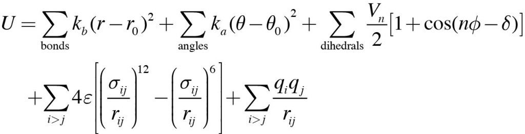
where the first through fifth terms on the right-hand side are the energies for bond stretching, angle bending, dihedral angle rotation, van der Waals interaction, and electrostatic interaction, respectively. The first three terms are also called bonded interactions, and the last two terms are called non-bonded interactions.
In the “atdyn” directory, you can see several files whose names start with “at_energy“. You can easily imagine that at_energy_bonds.fpp, at_energy_angles.fpp, at_energy_dihedrals.fpp, and at_energy_nonbonds.fpp are related to the energy calculation for the bond stretching, angle bending, dihedral angle rotation, and non-bonded interactions, respectively. As for the other files, we will not discuss them in detail here, since they are more advanced.
# List up the files related to the energy calculation
$ ls at_energy*.fpp
at_energy.fpp               at_energy_morph.fpp
at_energy_angles.fpp        at_energy_nonbonds.fpp
at_energy_bonds.fpp         at_energy_pme.fpp
at_energy_cg_nonlocal.fpp   at_energy_restraints.fpp
at_energy_dihedrals.fpp     at_energy_soft.fpp
at_energy_eef1.fpp          at_energy_str.fpp
at_energy_gamd.fpp          at_energy_table_cubic.fpp
at_energy_gbsa.fpp          at_energy_table_linear.fpp
at_energy_go.fpp            at_energy_table_linear_bondcorr.fpp
Now, let us focus on the bond stretching energy, as it is the simplest term in the above equation. The energy and force are given by
\( \normalsize{{U_{{\rm{bond}}}} = {k_b}{({r_{ij}} – {r_0})^2}} \)
\( \normalsize{{{\bf{F}}_j} = – 2{k_b}({r_{ij}} – {r_0})\frac{{{{\bf{r}}_{ij}}}}{{{r_{ij}}}}} \)
\( \normalsize{{\bf{F}}_i = – {\bf{F}}_j} \)
where kb is the force constant, rij is the distance between i-th and j-th atoms, and r0 is the equilibrium distance between the atoms. With these equations in mind, let’s take a look at at_energy_bond.fpp using the less command. According to the variable names and comment lines, you can indeed see that the distance between the atoms (r12), bond stretching energy (ebond), and force acting on each atom (force) are calculated from the atomic coordinates (coord), force constant (fc), and equilibrium distance (r0). For now you can just skim through the source code, since the main purpose of this tutorial is not to understand the source code in detail, but to get a quick idea of how the energy and force are calculated in GENESIS. To quit the less command, type “q” in the terminal window.
# Check the source code for the bond energy term (type "q" to quit)
$ less at_energy_bonds.fpp
  subroutine compute_energy_bond(enefunc, coord, force, virial, ebond)
:
    do i = istart, iend

      ! bond energy: E=K[b-b0]^2
      !
      d12(1:3) = coord(1:3,list(1,i)) - coord(1:3,list(2,i))
      r12   = sqrt( d12(1)*d12(1) + d12(2)*d12(2) + d12(3)*d12(3) )
      r_dif = r12 - r0(i)
      ebond = ebond + fc(i) * r_dif * r_dif

      ! gradient: dE/dX
      !
      cc_frc    = (2.0_wp * fc(i) * r_dif) / r12
      work(1:3,i) = cc_frc * d12(1:3)
:
    end do

    ! store force: F=-dE/dX
    !
    do i = istart, iend
      force(1:3,list(1,i)) = force(1:3,list(1,i)) - work(1:3,i)
      force(1:3,list(2,i)) = force(1:3,list(2,i)) + work(1:3,i)
    end do
If you are more interested in the source code for the energy and force calculations, please take a look at the contents of at_energy_angles.fpp, at_energy_dihedrals.fpp, and so on, as well as their parent module, at_energy.fpp. In fact, the parent subroutine in at_energy.fpp is called from within the do loop of the integrator, as explained next.
In which module are the atomic coordinates and velocities updated?
In MD simulation, the atomic coordinates and velocities are updated at each time step (Δt), which is repeated many times to realize the time evolution of the system. Such a protocol is called “time integration”. Typical integrators include the leap-frog algorithm and the velocity Verlet algorithm, both of which are available in atdyn. If you look in the atdyn directory, you can find at_md_leapfrog.fpp and at_md_vverlet.fpp. These modules are exactly related to the time integration. Here, we focus on the leap-frog algorithm, where the following two equations are solved iteratively.
\( \normalsize{{{\bf{v}}_i}(t + \frac{{\Delta t}}{2}) = {{\bf{v}}_i}(t – \frac{{\Delta t}}{2}) + \frac{{\Delta t}}{{{m_i}}}{{\bf{F}}_i}(t)} \)
\( \normalsize{{{\bf{r}}_i}(t + \Delta t) = {{\bf{r}}_i}(t) + \Delta t{{\bf{v}}_i}(t + \frac{{\Delta t}}{2})} \)
These equations give an NVE (microcanonical) ensemble to the system. Let’s take a look at at_md_leapfrog.fpp with the less command, and try to find the equations. You can see that there is a do loop with the comment “Main MD loop”, in which the two equations are solved iteratively. The following is an extract of the most important parts in the main MD loop.
# View the source code of the leapfrog integrator
$ less at_md_leapfrog.fpp
    ! Main MD loop
    !   coord is at 0 +  dt and vel is at 0 + 1/2dt, if restart off
    !   coord is at t + 2dt and vel is at t + 3/2dt, if restart on
    !
    do i = istart, iend
:
      ! Compute energy(t + dt), force(t + dt), and internal virial(t + dt)
      !
      call compute_energy(molecule, enefunc, pairlist, boundary, &
:
      ! Newtonian dynamics
      !   v(t+3/2dt) = v(t+1/2dt) + dt*F(t+dt)/m
      !   r(t+2dt)   = r(t+dt) + dt*v(t+3/2dt)
      !
      do j = 1, natom
        vel(1,j) = vel(1,j) + dt*force(1,j)*inv_mass(j)
        vel(2,j) = vel(2,j) + dt*force(2,j)*inv_mass(j)
        vel(3,j) = vel(3,j) + dt*force(3,j)*inv_mass(j)

        coord(1,j) = coord(1,j) + dt*vel(1,j)
        coord(2,j) = coord(2,j) + dt*vel(2,j)
        coord(3,j) = coord(3,j) + dt*vel(3,j)
      end do
:
      ! Output energy(t + dt) and dynamical variables(t + dt)
      !   coord     is at t +   2dt, coord_ref    is at t +    dt
      !   vel       is at t + 3/2dt, vel_ref      is at t + 1/2dt
      !   box_size  is at t +   2dt, box_size_ref is at t +    dt
      !
      call output_md(output, molecule, enefunc, dynamics, boundary, &
                     ensemble, dynvars)

    end do
Here, coord and vel are the atomic coordinates and velocities, respectively, dt is the time step, and inv_mass is the inverse of the atomic mass. As described above, the atomic forces are calculated in the subroutine “compute_energy“. The trajectories of the coordinates and energy are output in the subroutine “output_md“, which is contained in at_output.fpp.
In the case of the NVT or NPT ensemble, temperature and pressure are kept constant, where the velocities and coordinates are re-scaled according to the instantaneous temperature and pressure. In the leap-frog integrator of atdyn, Langevin thermostat/barostat [4,5] and Berendsen thermostat/barostat [6] are available. Let’s search for “langevin” or “berendsen” in at_md_leapfrog.fpp to see how the velocities and coordinates are re-scaled. In addition, let’s search for “constraints” to understand the SHAKE algorithm [7], which further updates the coordinates to fix the length of the covalent bond involving hydrogen.
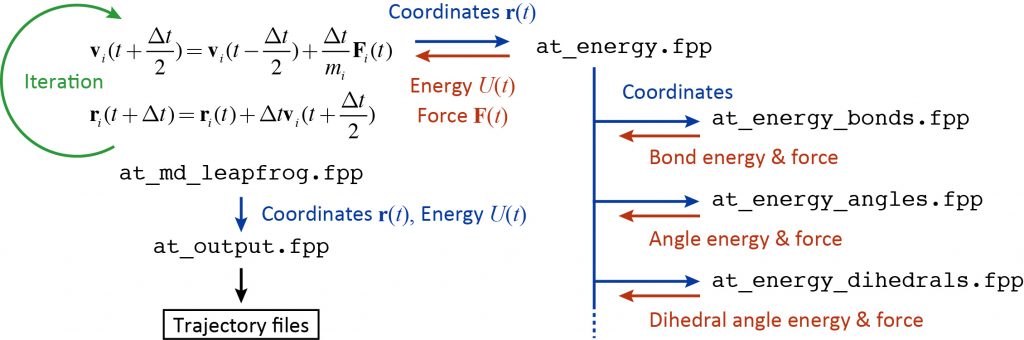
Overview of the core of MD simulation
The following figure summarizes the flowchart of the time integration, energy and force calculations, and trajectory output. Since GENESIS is a huge program package, it is not effective to read the source code from the beginning of the program. Rather, it is recommended to first understand the source code for energy and force calculations or time integration, which are the core of MD simulation. Then, you can expand your understanding of the source code based on your own knowledge of MD simulation such as the SHAKE algorithm, temperature and pressure controls. The MD program is indeed encoded with the theories you have learned in textbooks and literature.
References
- M. Tuckerman, “Statistical Mechanics: Theory and Molecular Simulation”, Oxford University Press (2010).
- M. P. Allen and D. J. Tildesley, “Computer Simulation of Liquids”, Oxford University Press (2017).
- D. Frenkel and B. Smit, “Understanding Molecular Simulation 2nd Edition”, Academic Press (2001).
- A. Brünger et al., Chem. Phys. Lett., 105, 495-500 (1984).
- S. E. Feller et al., J. Chem. Phys., 103, 4613-4621 (1995).
- H. J. C. Berendsen et al., J. Chem. Phys., 81, 3684-3690 (1984).
- J. P. Ryckaert et al., J. Comput. Phys., 23, 327-341 (1977).
Written by Takaharu Mori@RIKEN Theoretical molecular science laboratory
Jan. 3, 2022