15.1 Relative protein-ligand binding affinity
Contents
- 1. Relative binding affinity calculated by the free-energy perturbation method
- 2. Hybrid topology approach
- 3. Preparation for FEP simulations
- 4. Setup
- 5. ALCHEMY section
- 6. Minimization, heating, and equilibration
- 7. \(\lambda\)-exchange FEP simulation
- 8. Analysis
- 9. Embarrassingly parallel computing
- References
1. Relative binding affinity calculated by the free-energy perturbation method
The free-energy perturbation (FEP) method calculates the free-energy difference between two states using the following equation.
\( \displaystyle \Delta A = A_1 – A_0 \\ \displaystyle= – k_BT \ln \frac{\int dx \exp[-\beta U_1(x)]}{\int dx \exp[-\beta U_0](x)} \\ \displaystyle = – k_BT \ln \frac{\int dx \exp[-\beta U_0 (x)- \beta \Delta U(x)]}{\int dx \exp[-\beta U_0(x)]} \\ \displaystyle = – k_BT \ln \left<\exp[-\beta \Delta U(x)]\right>_0,\)
where \(A\) and \(U\) are the free energy and potential energy of state 0 or 1, and \(\Delta U\) is the difference between \(U_0\) and \(U_1\). This equation means that \(\Delta A\) can be estimated by sampling only equilibrium configurations of the state 0. However, if the difference between states 0 and 1 is large, there is little overlap of energy distributions (Left of Figure 1) and the configurations at state 1 are poorly sampled by simulations at the state 0, leading to large statistical errors. To reduce the errors, \(n-2\) intermediate states are inserted between states 0 and 1 to overlap energy distributions (Right of Figure 1). The potential energy of the intermediate state \(i\) is defined by \(U(\lambda_i) = (1-\lambda_i) U_0+\lambda_i U_1\), where \(\lambda_i\) is the scaling parameter for connecting the initial and final states. By changing \(\lambda_i\) from 0 to 1, states 0 and 1 can be connected smoothly. \(\Delta A\) can be estimated by calculating the summation of free-energy changes between adjacent states:
\( \displaystyle \Delta A = \sum_{i=0}^{n-1} \Delta A_i \\ \displaystyle= – k_BT \sum_{i=0}^{n-1} \ln \left<\exp[-\beta (U(\lambda_{i+1}) – U(\lambda_i)) \right>_{\lambda_i},\)
where the subscript \(\lambda_i\) represents the ensemble average at state \(i\).
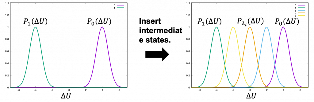
Figure 1. Distribution of energy differences and the stratification for them.
One of the most important applications of the FEP method is the calculation of protein-ligand binding affinity, which is defined as the free-energy change upon ligand binding. Here, we demonstrate how to calculate the relative binding affinity between two ligands for the system of FK506 Binding Protein (FKBP) [1] using the FEP method. The FKBP-ligand system is often used to benchmark the performance of a calculation method for protein-ligand binding affinities [2]. Figure 2 shows the thermodynamic cycle of FKBP binding with ligands L8 and L9. The relative binding affinity \(\Delta\Delta G\) is defined as the difference between the absolute binding affinities of two ligands: \(\Delta\Delta G = \Delta G_{binding}^{L9} – \Delta G_{binding}^{L8}\). In calculations of absolute binding affinities, the free-energy change from the bound state (the ligand fully interacts with the protein and solvent) to the unbound state (the ligand loses all interactions with the protein and solvent) must be calculated. However, in general, since the perturbation between the bound and unbound states is significantly large, a large number of intermediate states (usually more than 30 states) are required to keep statistical error within an acceptable range. In contrast, from the thermodynamic cycle in Figure 2, \(\Delta\Delta G\) can be calculated by the mutation from L8 to L9 instead of calculating \(\Delta G_{binding}^{L8}\) and \(\Delta G_{binding}^{L9}\):
\( \displaystyle \Delta\Delta G = \Delta G_{mutation}^{complex} – \Delta G_{mutation}^{ligand}\),
where \(\Delta G_{mutation}^{complex}\) and \(\Delta G_{mutation}^{ligand}\) are the free energy changes upon the mutation from L8 to L9 at the bound and unbound states, respectively. Since the perturbation in the mutation is small (from a benzene ring in L8 (green in Figure 2) to a cyclohexyl ring in L9 (magenta in Figure 2)), the number of intermediate states is reduced.
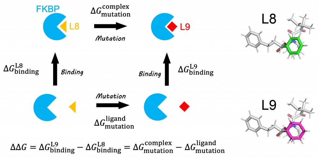
Figure 2. (Left) Thermodynamic cycle of protein-ligand binding and ligand mutation. (Right) L8 and L9.
2. Hybrid topology approach
Upon the mutation of L8 to L9, not only the molecular topology but also charge distribution changes. During FEP simulations, the force field parameters (partial charges, LJ parameters, etc.) should be gradually changed from L8’s parameters to L9’s by inserting intermediate states. To treat this change in the force field, we introduce the “hybrid topology approach” [3,4] to FEP simulations in this tutorial.
L8 and L9 have a common structure except for the benzene and cyclohexyl rings (green and magenta parts in Figure 3, respectively). A hybrid-topology structure is built by superimposing the common part (bottom of Figure 3). The superimposed part has a single topology, while the other part has a dual topology, in which the benzene and cyclohexyl rings coexist. They are hereafter referred to as the single-topology and dual-topology parts, respectively. During FEP simulations, the single-topology part does not change its topology, but its force field parameters (charge, LJ, and internal bond) are scaled by \(\lambda\). On the other hand, in the dual-topology part, the topology is changed as well as parameters. At the initial state (e.g. \(\lambda=0\)), only the benzene ring exists in the dual-topology part. As \(\lambda\) changes from 0 to 1, the benzene ring gradually disappears, whereas the cyclohexyl ring gradually appears. At the final state (e.g. \(\lambda=1\)), only the cyclohexyl ring exists in the dual-topology part. By these perturbations, the initial state (L8 structure) smoothly changes to final state (L9 structure)
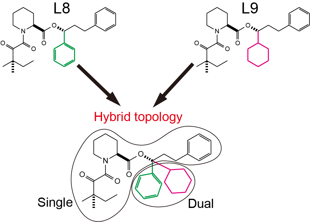
Figure 3. The topologies of L8 and L9 are merged into a hybrid topology.
3. Preparation for FEP simulations
Let’s start FEP simulations by employing FKBP-ligand systems as an example. First of all, let’s download the tutorial file (tutorial-15.1.tar). This tutorial consists of three directories: complex, ligand, and toppar. complex and ligand represent FEP simulations of the protein-ligand complex and those of the ligand in water, respectively. toppar includes files for force field parameters.
# Download the tutorial file
$ cd /home/user/GENESIS/Tutorials
$ mv ~/Downloads/tutorial-15.1.tar.gz ./
$ tar -xzvf tutorial-15.1.tar.gz
$ cd tutorial-15.1
$ ls
calc_ddG.py*  complex/  ligand/  toppar/
In “complex” directory, there are some script files and input files. run_min.inp, run_eq1.inp, run_eq2.inp, and run_eq3.inp are GENESIS control files for minimization, heating, equilibration with restraints, and long equilibration without restraints. make_inp.sh is a shell script for generation of control file for production run of FEP simulations. post_run.sh is a shell script for analysis. The “ligand” directory also includes input files similar to “complex” directory.
$ cd complex
$ ls
complex.pdb make_input.sh* post_run.sh* run_eq2.inp run_eq.sh* run_min.inp
complex.psf output/ run_eq1.inp run_eq3.inp run_fep.sh*
In this tutorial we learn how to calculate the relative binding affinity based on the CHARMM force field. However, the calculation can be also done using the AMBER forcefield. If you use the AMBER force field, please download the tutorial files for the AMBER force field (tutorial-15.1_amber.tar). The options in the GENESIS control files for the AMBER force field are almost the same as those for the CHARMM force field.
4. Setup
In GENESIS, the system for hybrid topology includes the whole structures of both L8 and L9 molecules in which the common parts of L8 and L9 (i.e., the single-topology part) are superimposed. That is, the common atoms of L8 and L9 are duplicated in the system (Figure 4). The duplication introduces unnecessary degrees of freedom and the error may occur if the coordinates and velocities of the common atoms in L8 become different from those in L9. In GENESIS, the additional degrees of freedom are removed and the coordinates and velocities of the common atoms are always synchronized during FEP simulations as if the common parts had no duplication.
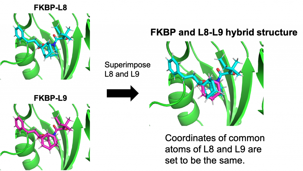
Figure 4. Representation of hybrid topology in GENESIS
An example of a PDB file is shown in Figure 5. The PDB file must contain the coordinates of ligands A and B, followed by those of protein and water. Each ligand is divided into single-topology and dual-topology parts. The single-topology and dual-topology parts of the initial state (L8: segment ID of L0) are respectively referred to as “single A” and “dual A”, while those of the final state (L9: segment ID of L1) are referred to as “single B” and “dual B”, respectively. The atom names, coordinates, and order of “single A” atoms must be the same as those of the “single B” atoms, because “single A” and “single B” parts are assumed to be the same in FEP simulations. The PSF file (or PRMTOP file for AMBER) corresponding to the PDB file is also required for FEP simulations.
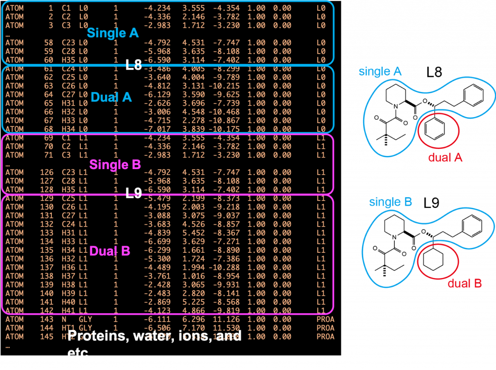
Figure 5. (Left) A PDB file for hybrid topology. (Right) Definitions of singleA, singleB, dualA, and dualB.
The PDB and PSF files for hybrid topology can be manually prepared, but it is very troublesome and mistakable. If there are even a little difference between the coordinates or the order of “single A” and “single B” atoms, GENESIS doesn’t work and stop the simulation. The bothering task can be alleviated using CHARMM-GUI. Relative Ligand Binder in CHARMM-GUI automatically prepares the PDB, PSF, and GENESIS input files for hybrid topology. A ligand can be easily mutated to the other ligand of interest using graphical user interface, and the force field parameters for the ligands are automatically generated using ParamChem. The PDB and PSF files in tutorial-15.1.tar.gz were generated using Relative Ligand Binder in CHARMM-GUI.
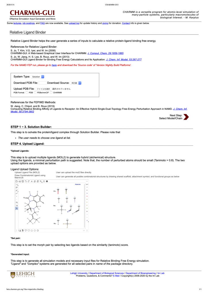
Figure 6. Front page of Relative Ligand Binder in CHARMM-GUI.
5. ALCHEMY section
Most of input options in the GENESIS control file are the same as explained in Tutorial 3.2, but [ALCHEMY] section is added to set the keywords related to FEP. To see options in [ALCHEMY] section, execute the following command:
# Show control options
$ /home/user/GENESIS/bin/spdyn -h ctrl_all md
All options in [ALCHEMY] section are shown below. fep_direction represents the direction of energy evaluation in FEP. BothSides, Forward, or Reverse are available. The topology in FEP simulations is specified by fep_topology (Hybrid or Dual). For hybrid topology, set fep_topology = Hybrid. The “single A”, “single B”, “dual A”, and “dual B” atoms of the ligands are assigned by keywords: singleA, singleB, dualA, and dualB, respectively. For these keywords, set the group numbers assigned in [SELECTION]. For example, if group1, group2, group3, and group4 are respectively assigned to “single A”, “single B”, “dual A”, and “dual B” atoms in [SELECTION] section, then set singleA = 1, singleB = 2, dualA = 3, and dualB = 4. fepout_period is the frequency of output of energy difference. It must be larger than or equal to eneout_period. equilsteps represents the equilibration steps before the evaluation of energy differences. In GENESIS, the soft-core potentials are applied to the LJ [5] and electrostatic [6] interactions between the dual-topology atoms and the others. sc_alpha and sc_beta are the parameters of soft-core potentials for LJ and electrostatic interactions, respectively. lambljA, lambljB, lambelA, lambelB, lambbondA, lambbondB, and lambrest represent values of \(\lambda\) for LJ, electrostatics, internal bonds, and restraints, respectively.
# [ALCHEMY]
# fep_direction = Bothsides             # Fep direction [Bothsides, Forward, Reverse]
# fep_topology  = Hybrid                # Fep topology [Hybrid, Dual]
# fep_md_type   = Serial                # FEP-MD or FEP-REMD [Serial, Single, Parallel]
# singleA       = 1                     # Group number for singleA atoms
# singleB       = 2                     # Group number for singleB atoms
# dualA         = 3                     # Group number for dualA atoms
# dualB         = 4                     # Group number for dualB atoms
# fepout_period = 100                   # output period for energy difference
# equilsteps    = 0                     # number of equilibration steps
# sc_alpha      = 5.0                   # LJ soft-core parameter
# sc_beta       = 0.5                   # Electrostatic soft-core parameter
# lambljA       = 1.0 0.75 0.5 0.25 0.0 # lambda for LJ in region A
# lambljB       = 0.0 0.25 0.5 0.75 1.0 # lambda for LJ in region B
# lambelA       = 1.0 0.75 0.5 0.25 0.0 # lambda for electrostatic in region A
# lambelB       = 0.0 0.25 0.5 0.75 1.0 # lambda for electrostatic in region B
# lambbondA     = 1.0 0.75 0.5 0.25 0.0 # lambda for internal bonds in singleA
# lambbondB     = 0.0 0.25 0.5 0.75 1.0 # lambda for internal bonds in singleB
# lambrest      = 1.0 1.0  1.0 1.0  1.0 # lambda for restraint energy
# ref_lambid    = 0                     # Reference window id for single FEP-MD
6. Minimization, heating, and equilibration
We carry out minimization and equilibration of the system with alchemical perturbation before a production run. First, we remove atomic clashes (or bad contacts) in the initial structure. The following command executes the minimization of the system:
# Perform minimization
$ /home/user/GENESIS/bin/spdyn -np 8 run_min.inp > output/run_min.out
The part of the control file for minimization is shown below. fep_direction, fepout_period, and equilsteps are not used in minimization, and they can be omitted. In [SELECTION] section, group1, group2, group3, and group4 are respectively assigned to “single A”, “single B”, “dual A”, and “dual B” atoms defined in Figure 5. We here set all values of lambljA, lambljB, lambelA, lambelB, lambbondA, and lambbondB to 1.0, which means that L8 and L9 molecules fully interacts with the other atoms in the system. lambrest can be omitted if the restraint is not scaled by \(\lambda\).
[ALCHEMY]
fep_topology = Hybrid
singleA      = 1 # Group number for singleA atoms
singleB      = 2 # Group number for singleB atoms
dualA        = 3 # Group number for dualA atoms
dualB        = 4 # Group number for dualB atoms
sc_alpha     = 5.0
sc_beta      = 0.5
lambljA      = 1.0
lambljB      = 1.0
lambelA      = 1.0
lambelB      = 1.0
lambbondA    = 1.0
lambbondB    = 1.0

…

[SELECTION]
group1 = ai:1-60 and segid:L0    # group for singleA atoms
group2 = ai:69-128 and segid:L1  # group for singleB atoms
group3 = ai:61-68 and segid:L0   # group for dualA atoms
group4 = ai:129-142 and segid:L1 # group for dualB atoms
Next, we heat up the system from 0.1 K to 300 K. The following command executes the heating of the system:
# Perform heating
$ /home/user/GENESIS/bin/spdyn -np 8 run_eq1.inp > output/run_eq1.out
In FEP MD simulations, the energy difference (\(\Delta U\)) between two states are calculated. \(\lambda\) values for each state are specified by a column in lambljA, lambljB, lambelA, lambelB, lambbondA, and lambbondB. In the control file shown below, two columns of \(\lambda\) values correspond to the states. When ‘Forward’ is specified in fep_direction, GENESIS performs a FEP simulation only at state 1 (left column of \(\lambda\) values) and calculate the energy difference between states 1 and 2 (right column of \(\lambda\) values) at state 1. The energy difference is outputted to ‘fepfile’ specified in [OUTPUT]. In this example, \(\lambda\) values of states 1 and 2 are the same, so that the energy difference is 0.
[OUTPUT]
dcdfile = output/run_eq1.dcd
rstfile = output/run_eq1.rst
fepfile = output/run_eq1.fepout

[ALCHEMY]fep_direction = Forward
fep_topology  = Hybrid
singleA       = 1
singleB       = 2
dualA         = 3
dualB         = 4
fepout_period = 0
equilsteps    = 0
sc_alpha      = 5.0
sc_beta       = 0.5
lambljA       = 1.0 1.0
lambljB       = 1.0 1.0
lambelA       = 1.0 1.0
lambelB       = 1.0 1.0
lambbondA     = 1.0 1.0
lambbondB     = 1.0 1.0
Subsequently, we perform NPT equilibration with restraints (100 ps) and long NPT equilibration without restraints (1 ns). In those simulations, [ALCHEMY] is the same as the heating. After the simulations, please check the log files and watch the trajectories using VMD.
# Perform equilibration with positional restraints
$ /home/user/GENESIS/bin/spdyn -np 8 input/run_eq2.inp > output/run_eq2.out

# Perform equilibration without the restraints
$ /home/user/GENESIS/bin/spdyn -np 8 input/run_eq3.inp > output/run_eq3.out
7. \(\lambda\)-exchange FEP simulation
In this step, we perform the production run of FEP simulations. To enhance the sampling efficiency, the FEP simulations at different \(\lambda\) values are coupled using the Hamiltonian replica exchange method [7,8]. We prepare 12 replicas in this tutorial. Two of them corresponds to the initial and final states, while the other 10 replicas correspond to intermediate states. 12 replicas run in parallel and exchange their parameters at fixed intervals during the simulation. Exchanges between adjacent replicas are accepted or rejected according to Metropolis’s criterion.
The following command generates input files for \(\lambda\)-exchange FEP simulations:
# Execute the shell script for generation of input files
$ sh make_inp.sh
This script generates five input files (run_fep1.inp to run_fep5.inp). Each file is for a 1-ns FEP simulation. By using them in a sequential order, we can perform 5-ns simulations in total. For convenience in this tutorial, we here use only run_fep1.inp (i.e., only a 1-ns simulation is performed).
The following command executes the simulation:
# Execute the control file for the lambda-exchange FEP simulation
# 8 MPI processes per replica, i.e. 8 * 12 = 96 processes are used here
$ /home/user/GENESIS/bin/spdyn -np 96 input/run_fep1.inp > output/run_fep1.out
The most important parts in run_fep1.inp are shown below. In the \(\lambda\)-exchange FEP simulation, [REMD] section is also required. type1 is set to alchemy to exchange \(\lambda\) values. exchange_period should be multiples of fepout_period. In [ALCHEMY] section, fep_direction is set to ‘Bothsides’. If ‘Bothsides’ is specified, the energy differences between adjacent replicas are calculated in each replica. For example, consider replica i. The energy differences between i and i-1 and between i and i+1 are calculated and outputted to the file specified by ‘fepfile’ at the fixed intervals specified by ‘fepout_period’. Figure 7 shows an example of fepfile of replica 2 (window 2). The fepfile are used to calculate the free energy in next section “8. Analysis”. The \(\lambda\) values for each replica are specified by lambljA, lambljB, lambelA, lambelB, lambbondA, and lambbondB. The leftmost column of the \(\lambda\) values corresponds to the parameters for the initial state (i.e., L8), the rightmost column corresponds to the parameters for the final state (i.e., L9), and the other columns correspond to the parameters for the intermediate states. In this tutorial, we change lambljA, lambljB, lambelA, lambelB, lambbondA, and lambbondB along replica IDs as shown in Figure 8.
[REMD]
dimension = 1
exchange_period = 800
type1 = alchemy
nreplica1 = 12

[ALCHEMY]
fep_direction = BothSides
fep_topology = hybrid
singleA = 1
singleB = 2
dualA   = 3
dualB   = 4
fepout_period = 400
equilsteps = 0
sc_alpha   = 5.0
sc_beta    = 5.0
lambljA    = 1.0   0.909 0.818 0.727 0.636 0.545 0.455 0.364 0.273 0.182 0.091 0.0
lambljB    = 0.0   0.091 0.182 0.273 0.364 0.455 0.545 0.636 0.727 0.818 0.909 1.0
lambelA    = 1.0   0.909 0.818 0.727 0.636 0.545 0.455 0.364 0.273 0.182 0.091 0.0
lambelB    = 0.0   0.091 0.182 0.273 0.364 0.455 0.545 0.636 0.727 0.818 0.909 1.0
lambbondA  = 1.0   0.909 0.818 0.727 0.636 0.545 0.455 0.364 0.273 0.182 0.091 0.0
lambbondB  = 0.0   0.091 0.182 0.273 0.364 0.455 0.545 0.636 0.727 0.818 0.909 1.0
lambrest   = 1.0   1.0   1.0   1.0   1.0   1.0   1.0   1.0   1.0   1.0   1.0   1.0

Figure 7. Example of fepfile.
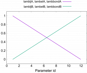
Figure 8. Values of \(\lambda\) for electrostatic, LJ, and bonded interactions.
For convenience, we here perform only a 1-ns \(\lambda\)-exchange FEP simulation using the rRESPA integrator with 2.5-fs time step. However, it might not be sufficient to converge the free-energy calculation. If you have enough computational resource or time, you should run longer simulations to obtain better results.
8. Analysis
We calculate the free energy from fepfile obtained by the \(\lambda\)-exchange FEP simulation. The following command calculates the free-energy difference between the initial and final states:
# Execute the shell script for analysis
$ sh post_run.sh
The part of post_run.sh is shown below. This script first sorts fepfile to output the energy differences for each parameter (\(\lambda\)) (par1.fepout to par12.fepout) using remd_convert, which is included in GENESIS analysis tools. Second, the free-energy differences between adjacent parameter sets are calculated from the sorted files using the Bennett acceptance ratio (BAR) method. The BAR method is performed using mbar_analysis in GENESIS analysis tools. The number of simulations, the number of replicas, the number of steps, the frequency of replica exchange, the frequency of energy output, and temperature are specified by nrun, nrep, nsteps, exchange_period, fepout_period, and temperature, respectively. The simulations from ini-th to fin-th are used for analysis. For example, in the below script, only the first run is used (i.e., run1 to run1). Please adapt these parameters to the user’s requirements. Also, GENESIS_BIN_DIR must be set to the path for GENESIS analysis tools. By executing post_run.sh, we obtain fene.dat including the free-energy differences along the parameter IDs.
# set parameters of simulations
nrun=1
nrep=12
nsteps=400000
exchange_period=800
fepout_period=400
temperature=300
ini=1
fin=$nrun

# set path for genesis analysis tools
GENESIS_BIN_DIR=
Figure 9 shows the free-energy changes from the initial state (L8: Parameter 1) to the final state (L9: Parameter 12). The difference between the initial and final states for the protein-ligand complex and that for the isolated ligand in water correspond to \(\Delta G_{mutation}^{complex}\) and \(\Delta G_{mutation}^{ligand}\), respectively. From our calculations, we obtained \(\Delta G_{mutation}^{complex}= -10.20 ± 0.19\) kcal/mol and \(\Delta G_{mutation}^{ligand} = -10.05 ± 0.19\) kcal/mol. Therefore, the relative binding affinity of L8 and L9 is \(\Delta\Delta G = -0.15 ± 0.27\) kcal/mol, which is in good agreement with the experimental results (0.2 kcal/mol) [1].
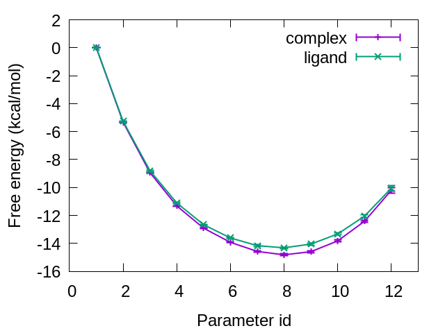
Figure 9. Free-energy changes from the initial state to the final state for complex and ligand.
9. Embarrassingly parallel computing
\(\lambda\)-exchange FEP requires large computational resource at one time, because MD simulations for all \(\lambda\) windows must be performed simultaneously and be exchanged periodically. However, if the replica-exchange is not used or not needed for our calculations, \(\lambda\) windows become independent each other, and simulations for different \(\lambda\) can be performed separately. This parellization is called “embarrasingly parallel” (also called “bakapara” in Japanese).To generate input files for embarrasingly parallel FEP simulations, comment out md_type=remd and uncomment md_type=distributed in make_inp.sh.
# set md type (remd or distributed)
#md_type=remd
md_type=distributed
make_inp.sh generates 60 input files (run1_rep1.inp to run1_rep12.inp, run2_rep1.inp to run2_rep12.inp, …). run1_rep1.inp is for the 1-ns FEP simulation with only window’s ID 1. The part in run1_rep1.inp is shown below. In this input file, [REMD] section is removed. fep_md_type and ref_lambid are added in [ALCHEMY] section. When fep_md_type is set to Single, the simulation uses only one lambda window and becomes embarrassingly parallel. ref_lambid specifies the lambda windows used for the simulation.
[ALCHEMY]
fep_direction = BothSides
fep_topology = hybrid
fep_md_type = Single
ref_lambid = 1
singleA = 1
singleB = 2
dualA = 3
dualB = 4
...
MD simulations with run1_rep1.inp to run1_rep12.inp can be performed independently. By using them in a sequential order (i.e., run2_rep*.inp, run3_rep*.inp, …), we can perform 5-ns simulations in total.
In embarrassingly parallel compuation, we don’t need to sort fepfile using remd_convert. To obtain the free-energy difference, comment out md_type=remd and uncomment md_type=distributed in post_run.sh, which avoid sorting and concatenate fepfile obtained by FEP simulations.
References
- D. A. Holt, J. I. Luengo, D. S. Yamashita, H. J. Oh, A. L. Konialian, H. K. Yen, L. W. Rozamus, M. Brandt, M. J. Bossard, Design, Synthesis, and Kinetic Evaluation of High-Affinity FKBP Ligands and the X-Ray Crystal Structures of Their Complexes with FKBP12. J. Am. Chem. Soc. 115, 9925–9938 (1993).
- H. Fujitani, Y. Tanida, and A. Matsuura, Massively parallel computation of absolute binding free energy with well-equilibrated states. Phys. Rev. E 79, 021914 (2009).
- J. W. Kaus, L. T. Pierce, R. C. Walker, and J. A. McCammon, Improving the Efficiency of Free Energy Calculations in the Amber Molecular Dynamics Package. J. Chem. Theory Comput. 9, 4131–4139 (2013).
- W. Jiang, C. Chipot, and B. Roux, Computing Relative Binding Affinity of Ligands to Receptor: An Effective Hybrid Single-Dual-Topology Free-Energy Perturbation Approach in NAMD. J. Chem. Inf. Model. 59, 3794–3802 (2019).
- M. Zacharias, T. P. Straatsma, and J. A. McCammon, Separation‐shifted scaling, a new scaling method for Lennard‐Jones interactions in thermodynamic integration. J. Chem. Phys. 100, 9025–9031 (1994).
- T. Steinbrecher, I. Joung, and D. A. Case, Soft-core potentials in thermodynamic integration: Comparing one- and two-step transformations. J. Comput. Chem. 32, 3253–3263 (2011).
- Y. Sugita, A. Kitao, and Y. Okamoto, Multidimensional Replica-Exchange Method for Free-Energy Calculations. J. Chem. Phys. 113, 6042–6051 (2000).
- H. Fukunishi, O. Watanabe, S. Takada, On the Hamiltonian Replica Exchange Method for Efficient Sampling of Biomolecular Systems: Application to Protein Structure Prediction. J. Chem. Phys. 116, 9058−9067 (2002).
Written by Hiraku Oshima@RIKEN BDR
September 6, 2021