16.2 Multi-scale cryo-EM flexible fitting
MD-based flexible fitting to the cryo-electron microscopy (Cryo-EM) density map at a resolution close to 5 Å is challenging, when a protein domain has to undergo a sophisticated conformational change, such as domain rotation. The protocol presented here and described in [1] involves a few steps, that significantly increase the chances for the correct fitting in such difficult cases. It employs the replica-exchange flexible fitting to obtain a correct protein movement/rotation [2]. To speed up the calculations, the coarse-grained Go-model developed by Karanicolas and Brooks (KB Go-model) [3,4] is used at this step. Then, to map the coarse-grained model to the full-atom model, the targeted MD method is used. Finally, the obtained structure is refined with the all-atom MD flexible fitting [5].
Before going through this tutorial, it is advised to complete the basic tutorials concerning the basic MD-based flexible fitting protocol (Tutorial 16.1), the MD simulations using the GB/SA model (Tutorial 8.1), the coarse-grained MD simulations using the KB Go-model (Tutorial 7.1) and the replica-exchange MD (REMD) simulations (Tutorial 12.1).
Preparation
The tutorial files are available for download here: tutorial22-16.2.zip. As described in Tutorial 16.1, installing the SITUS program package and making a symbolic link to the CHARMM toppar directory is necessary.
$ cd Tutorials
$ mv ~/Downloads/tutorial22-16.2.zip ./
$ unzip tutorial22-16.2.zip
$ cd tutorial-16.2
$ ln -s ../../Others/CHARMM/toppar ./
$ ls
01_CG_emmap      02_CG_build    03_CG_REMD_fitting  04_CG_analysis
05_AA_emmap      06_AA_build    07_AA_minimize      08_AA_targeted_MD
09_AA_refinement 10_AA_analysis toppar
1. Coarse-grained (CG) simulations
1.1. Preparing a simulated density map of the target state
In this tutorial, a small protein (adenylate kinase) in open state will be fitted to a simulated density map in the closed state. First, the density map for the coarse-grained simulations will be generated as the target for the fitting, basing on the PDB: 1AKE. Downloading and modifying the PDB file is necessary, so that the structure contains only protein chain A with non-hydrogen atoms:
# Download the PDB file of the closed state of adenylate kinase
$ cd 01_CG_emmap
$ wget https://files.rcsb.org/download/1AKE.pdb

# Generate a new PDB file that contains protein heavy atoms
$ vmd -dispdev text 1AKE.pdb
vmd > set sel [atomselect top "chain A and protein and not hydrogen and not altloc B"]
vmd > $sel writepdb closed.pdb
vmd > exit
The synthetic density map is generated by the emmap_generator with the provided INP file and should be visualized in VMD, as described in Tutorial 16.1.
# Generate synthetic EM density map (CG_closed.sit)
$ /home/user/GENESIS/bin/emmap_generator INP > log
1.2. Building the initial structure
The structure of adenylate kinase in the open state should be downloaded and modified in the same fashion as it was done with structure in the closed state:
# Download PDB file of the open state of adenylate kinase
$ cd ../02_CG_build/
$ wget https://files.rcsb.org/download/4AKE.pdb
$ ls
4AKE.pdb

# Generate a new PDB file that contains protein heavy atoms
$ vmd -dispdev text 4AKE.pdb
vmd > set sel [atomselect top " chain A and protein and not hydrogen and not altloc B"]
vmd > $sel writepdb open.pdb
vmd > exit
Now, it is possible to visualize the open.pdb in VMD, together with the situs map CG_closed.sit. The structure of adenylate kinase in the open state is shifted from the map, so the initial rigid body fitting step with colores is necessary:
# Perform rigid-body fitting using SITUS
$ /home/user/Situs_3.1/bin/colores ../01_CG_emmap/CG_closed.sit open.pdb -res 5 -nprocs 4
This calculation results in 7 new col_*.pdb files with fitted structures. For further calculations, we should choose the structure with the highest cross-correlation coefficient (c.c.) between the fitted structure and simulated densities:
# Check the c.c. value in the obtained PDB files
$ grep "Unnormalized correlation coefficient:" col_*.pdb
col_best_001.pdb:REMARK    Unnormalized correlation coefficient: 0.709285
col_best_002.pdb:REMARK    Unnormalized correlation coefficient: 0.614500
col_best_003.pdb:REMARK    Unnormalized correlation coefficient: 0.601603
col_best_004.pdb:REMARK    Unnormalized correlation coefficient: 0.590259
col_best_005.pdb:REMARK    Unnormalized correlation coefficient: 0.590186
col_best_006.pdb:REMARK    Unnormalized correlation coefficient: 0.580958
col_best_007.pdb:REMARK    Unnormalized correlation coefficient: 0.562662
As a result, col_best_001.pdb will be used as the initial structure to generate the coarse-grained KB Go-model parameters. For this purpose, we will use the MMTSB Web Service, as described in details in the Tutorial 7.1: Coarse-grained MD simulation with the KB Go-model. First, we should prepare the col_best_001.pdb file for the submission to the server:
# "clean" the file by deleting the entries other than ATOM
$ grep -e "^ATOM" col_best_001.pdb  > col_best_001_edited.pdb
Next, we submit it to the MMTSB server, with a reference tag (i.e. open). The tar-ball file is sent to your email address. We unpack it in the working directory:
# extract the tar-ball file
$ tar -xvf open.tar
To build the Go-model for simulations, several modifications have to be applied to the files from MMTSB, such as replacing the atom names. Superimposing the coordinates of molecule in GO_open.pdb file on the original coordinates submitted to the server can be done using the CA atoms positions. Then it is possible to generate the go.psf and go.pdb files for the CG simulation using VMD. For the details, please see Tutorial 7.1. This is done with the provided setup.tcl script:
##### read pdb
mol load pdb GO_open.pdb
mol load pdb col_best_001_edited.pdb

##### calculate the shift matrix using the CA atoms positions
set base_shifted [atomselect 0 "name CA"]
set base_original [atomselect 1 "name CA"]
set matrix [measure fit $base_shifted $base_original]

##### move the  GO_open.pdb structure
set shifted_molecule [atomselect 0 "all"]
$shifted_molecule move $matrix

##### replace residue names with G1, G2, G3, ...
set residue_list [lsort -unique [$shifted_molecule get resid]]
foreach i $residue_list {
    set resname_go [format "G%d" $I]
    set res [atomselect 0 "resid $i" frame all]
    $res set resname $resname_go
}
$shifted_molecule writepdb tmp.pdb

##### generate PSF and PDB files
package require psfgen
resetpsf
topology GO_open.top

segment PROT {
 first none
 last none
 pdb tmp.pdb
}

regenerate angles dihedrals
coordpdb tmp.pdb PROT

# write psf and pdb files
writepsf go.psf
writepdb go.pdb

exit
The script can be run with VMD:
$vmd -dispdev text <setup.tcl | tee run.out
The structure should be visually inspected. The positions of coordinates should coincide with the density map, so it is worth to open and see also the ../01_CG_emmap/CG_closed.sit in VMD:
$ vmd -situs ../01_CG_emmap/CG_closed.sit
vmd > mol load pdb go.pdb psf go.psf
1.3. Flexible fitting with replica-exchange scheme
When using the coarse-grained models, it is not necessary to run minimization and equilibration. We can run the production step immediately. For real applications, all the simulations shown in this tutorial should have more time steps to achieve a better convergence. The input file for the production run using 32 replicas is provided in the next folder:
# Change directory to run the CG simulation
$ cd ../03_CG_REMD_fitting
$ ls
INP
Have a look at the parameters provided in the INP file, both for REMD and flexible fitting parts:
[INPUT]
topfile = ../02_CG_build/GO_open.top       # topology file
parfile = ../02_CG_build/GO_open.param     # parameter file
psffile = ../02_CG_build/go.psf            # protein structure file
pdbfile = ../02_CG_build/go.pdb            # PDB file

[OUTPUT]
dcdfile         = md_{}.dcd
rstfile         = md_{}.rst
logfile         = log_{}.log
remfile         = md_{}.rem

[ENERGY]
forcefield      = KBGO         # [CHARMM,GO]
electrostatic   = CUTOFF       # [CUTOFF,PME]
switchdist      = 18.0         # switch distance
cutoffdist      = 20.0         # cutoff distance
pairlistdist    = 21.5         # pairlist distance

[DYNAMICS]
integrator      = LEAP         # [LEAP,VVER]
nsteps          = 1000000      # number of MD steps for 20ns
timestep        = 0.02         # timestep (ps)
eneout_period   = 100          # output energy
crdout_period   = 10000
rstout_period   = 1000000
nbupdate_period = 10           # update nonbond list
iseed           = 1

[REMD]
dimension       = 1
exchange_period = 100
iseed           = 1
type1           = RESTRAINT
nreplica1       = 32
cyclic_params1  = NO
rest_function1  = 1

[CONSTRAINTS]
rigid_bond      = YES          # constraints all bonds
fast_water      = NO           # settle constraint
shake_tolerance = 1.0e-6       # tolerance (Angstrom)

[ENSEMBLE]
ensemble        = NVT          # [NVE,NVT,NPT,NPAT]
tpcontrol       = BERENDSEN    # [NO,BERENDSEN,NOSE-HOOVER,LANGEVIN,GAUSS] for [LEAP]
temperature     = 200          # initial temperature (K)
tau_t           = 1.0          # thermostat friction (ps-1) in [LANGEVIN]

[BOUNDARY]
type            = NOBC

[SELECTION]
group1          = all

[RESTRAINTS]
nfunctions      = 1
function1       = EM
constant1 = 500 524 555 593 636 684 737 794 856 921 991 1065 1144 1228 1318 1415 1519 \
            1632 1755 1889 2035 2195 2371 2564 2777 3011 3269 3553 3865 4209 4586 5000
select_index1   = 1

[EXPERIMENTS]
emfit           = YES
emfit_target    = ../01_CG_emmap/CG_closed.sit
emfit_sigma     = 2.5         # Sigma in simulated map definition
emfit_tolerance = 0.01        # Tolerance for simulated map calculation
emfit_period    = 1           # update of the force
The set of 32 force constants provided here was previously tested in reference [1] to ensure sufficient overlaps between the potential energies of replicas and, as a result, the exchange ratios in the range of 0.2 – 0.3 for most of the studied protein systems. The exchange period (100) was also previously tested and yielded better results for tested proteins than exchange periods 10 or 1000. Note, that by decreasing the exchange period to 0 you can automatically perform 32 independent fitting runs at different force constants.
Now, we are ready to execute mpirun using 64 CPU cores (the number of CPU cores should be a multiplication of the number of replicas). This calculation may take a few hours and should be submitted as a batch job on the cluster.
# Perform REMD flexible fitting
$ export OMP_NUM_THREADS=2
$ mpirun -np 32 /home/user/GENESIS/bin/atdyn INP > log
Many files are produced as a result of the simulation: md_*.dcd, md_*.rem, md_*.rst, log_*.log for each replica * and log. The log_*.log files contain information about time course of the energy and c.c. of each replica. After the fitting, it is necessary to visualize at least one trajectory with VMD to ensure that the structure is well fitted to the target density.
$ vmd -situs ../01_CG_emmap/CG_closed.sit
vmd > mol load pdb ../02_CG_build/go.pdb psf ../02_CG_build/go.psf
vmd > mol addfile md_1.dcd
1.4. Analysis of the fitting results
It is time to analyze the changes in c.c. during the simulation, saved in the column 14: RESTR_CVS001 in the log_*.log files. It can be done simultaneously for all 32 replicas in a “for” loop with a simple bash script, provided in the tutorial files. This script also shows which replica have given the highest c.c. Have a look at the script:
#!/bin/sh

for REP in `seq 1 32`
    do
    grep 'INFO:' ../03_CG_REMD_fitting/log_${REP}.log | awk '{printf ("%10s\t%20s\n",$2,$15)}' | grep -v "RESTR"  > temp1
    awk -v var=log_${REP}.log '{print var,"\t",$0}' temp1 > cc-list$REP
    rm temp1
    highest_cc=$(awk '{print $3}' cc-list$REP | sort -n | tail -1)
    grep "$highest_cc" cc-list$REP  >> temp2
done

sort -rk3 temp2 > the-highest-cc.txt
rm temp2
We run the bash script in the following way:
# Change directory for analysis
$ cd ../04_CG_analysis

# Run the bash script
$ chmod +x analyze-cc.sh
$ ./analyze-cc.sh
The script generates a series of files cc-list* for each replica and a single file the-highest-cc.txt. All files contain the log name in the first column, time step in the second column, and c.c. in the last column.
1.5. Choosing the model with the highest cross-correlation coefficient
The file the-highest-cc.txt gathers the highest c.c. values from all replicas and it is sorted according to the c.c. value in the last column:
log_1.log                   634300                      0.9065
log_15.log                 223000                      0.9064
log_11.log                 623100                      0.9064
log_5.log                   248000                      0.9063
log_8.log                   316300                      0.9062
...
It is visible that the replica 1 reached the highest c.c. 0.9065 in the time step 634300. Thus, we encourage the users to calculate the RMSD and to generate a graph “Time courses of c.c. and Cα RMSD with respect to the target structure” for replica 1 by yourself. This can be done in a very similar way as it was described in the Tutorial 17.1.
For the targeted MD simulation, the frame from the REMD simulation that has the highest c.c. has to be extracted from the trajectory:
$ vmd -dispdev text
vmd > mol load pdb ../02_CG_build/go.pdb psf ../02_CG_build/go.psf
vmd > mol addfile ../03_CG_REMD_fitting/md_1.dcd
vmd > animate write pdb CG_open.pdb beg 63 end 63
vmd > exit
2. All atom (AA) simulations
2.1. Preparing a simulated density map of the target state
The simulated density map for the AA simulations is prepared in a similar way as for CG simulations, but a smaller voxel size is used. The synthetic density map is again generated with the emmap_generator and should be visualized.
# Change directory
$ cd ../05_AA_emap

# Generate synthetic EM density map (AA_closed.sit)
$ /home/user/GENESIS/bin/emmap_generator INP > log
2.2. Building the initial structure
We use the best structure fitted with Situs (../02_CG_build/col_best_001.pdb) as the initial coordinates for the targeted MD simulation. Here, we use the CHARMM force field and the initial pdb and psf files can be prepared with VMD as in Tutorial 2.3:
$ cd ../06_AA_build

$ vmd -dispdev text
vmd > package require psfgen
vmd > resetpsf
vmd > topology ../toppar/top_all36_prot.rtf
vmd > pdbalias residue HIS HSD
vmd > pdbalias atom ILE CD1 CD
vmd > segment PROA {pdb ../02_CG_build/col_best_001.pdb}
vmd > coordpdb ../02_CG_build/col_best_001.pdb  PROA
vmd > guesscoord
vmd > writepdb open.pdb
vmd > writepsf open.psf
vmd > exit
Now, it is time to prepare the target pdb file for the targeted MD simulation. We will use the MD frame with the highest c.c. derived in section 1.5. Choosing the model with the highest cross-correlation coefficient. Unfortunately, this MD frame does not have any other atoms than CA and the target pdb in GENESIS needs to have the same number of atoms as the pdb file used in this simulation, even if we select only the CA atoms as a target. Therefore, we copy the open.pdb file, substitute the coordinates of the CA atoms with the coordinates from the CG_open.pdb and save the new “fake” pdb file as CG_open2.pdb. The bash script prepare-target.sh for this operation is given in the folder 06_AA_build.
# Run the bash script
$ chmod +x prepare-target.sh
$ ./prepare-target.sh
2.3. Energy minimization
Before the targeted MD simulation, the structure needs to undergo energy minimization to remove steric clashes. The input file for this calculation is provided.
# Perform energy minimization using 16 CPU cores
$ cd ../07_AA_minimize
$ export OMP_NUM_THREADS=4
$ mpirun -np 4 /home/user/GENESIS/bin/atdyn INP > log
2.4. Targeted MD towards the chosen model from CG simulations
Next, we perform the targeted MD in implicit solvent.
# Change directory to run targeted MD
$ cd ../08_AA_targeted_MD
The control file is given in the folder. For the targeted simulation, the CA atoms are chosen:
[SELECTION]
group1           = an:CA

[RESTRAINTS]
nfunctions       =        1
function1        =     RMSD
constant1        =      500
reference1       =        0
select_index1    =        1

[FITTING]
fitting_method   = TR+ROT
fitting_atom     = 1
mass_weight      = NO
Now it is necessary to extract the last frame from the targeted fitting. Also, after the targeted MD, the structure might be still shifted a little with respect to the positions of the CA atoms. This is why we additionally superimpose the obtained structure on the CA positions after REMD fitting in VMD with the provided setup.tcl script:
##### save the last frame
mol load pdb ../06_AA_build/open.pdb psf ../06_AA_build/open.psf
mol addfile md.dcd
animate write pdb targeted_last.pdb beg last end last
mol delete all

##### read pdb
mol load pdb targeted_last.pdb
mol load pdb ../06_AA_build/CG_open2.pdb

##### calculate the shift matrix using the CA atoms positions
set base_shifted [atomselect 1 "name CA"]
set base_original [atomselect 2 "name CA"]
set matrix [measure fit $base_shifted $base_original]

##### move the  targeted_last.pdb structure
set shifted_molecule [atomselect 1 "all"]
$shifted_molecule move $matrix
$shifted_molecule writepdb targeted_shifted.pdb

exit
Let’s visualize the targeted MD trajectory with VMD. We need to check if the CA atoms in targeted_shifted.pdb are well fitted to the CA positions from the KB Go-model simulations and how big is the difference in CA positions before and after the superimposing:
$ vmd -pdb ../06_AA_build/open.pdb ../06_AA_build/open.psf md.dcd
vmd > mol load pdb targeted_shifted.pdb
vmd > mol load pdb ../04_CG_analysis/CG_open.pdb
2.5. Refinement of the structure with flexible fitting
The last step of the multi-scale protocol involves the refinement of the obtained fitted model with the MD flexible fitting using CHARMM force field in implicit solvent. The control file is also provided in the directory.
# Change directory to run the MD fitting
$ cd ../09_AA_refinement
The biasing potential set on the protein heavy atoms is very high, because the protein is already fitted to the density and we want to refine the positions of the side chains. See the part of the input file responsible for the fitting:
[SELECTION]
group1          = all and heavy

[RESTRAINTS]
nfunctions      = 1
function1       = EM
constant1       = 20000
select_index1   = 1

[EXPERIMENTS]
emfit           = YES
emfit_target    = ../05_AA_emmap/AA_closed.sit
emfit_sigma     = 2.5        # Sigma in simulated map definition
emfit_tolerance = 0.01       # Tolerance for simulated map calculation
emfit_period    = 1          # update of the force
The MD flexible fitting simulation can be executed with ATDYN using 16 CPU cores:
# Perform flexible fitting
$ export OMP_NUM_THREADS=4
$ mpirun -np 4 /home/user/GENESIS/bin/atdyn INP > log
The files run.dcd, run.pdb, run.rst and log are produced during the simulation.
2.6. Analysis of the fitting results
The RMSD with respect to the target structure, the time course of c.c. and MolProbity score can be easily analyzed for the MD flexible fitting refinement trajectory. However, this was already described in details in Tutorial 17.1 so the users are advised to do those analyses by themselves.
# Change directory for analysis
$ cd ../10_AA_analysis
Here, we find the highest value of c.c. in the final simulation. The following commands extract the time step (first column) and c.c. value (second column) and sort according to the c.c. value:
# Find the highest c.c.
$ grep "INFO:" ../09_AA_refinement/log| awk '{print $2, $19}' | grep -v "RESTR" > cc.log

$ sort -rk 2 cc.log | head -5
39500 0.9840
47000 0.9837
46500 0.9837
34000 0.9837
48500 0.9836
The structure characterized with the highest c.c. is supposed to be the best structure obtained in the fitting simulation. It is reached at the 39500 time step with the crdout_period = 500, so it will be the 79th frame in the trajectory. Let’s extract this structure from the trajectory and compare it with the initial structure and the best structures obtained in the CG REMD fitting and in targeted MD. We should also visualize the trajectory in VMD to see how well the structure fits the density:
# Find the best fitted structure after the MD refinement
$ vmd -situs ../05_AA_emmap/AA_closed.sit
vmd > mol load pdb ../06_AA_build/open.pdb psf ../06_AA_build/open.psf
vmd > mol addfile ../09_AA_refinement/md.dcd
vmd > animate write pdb final_best.pdb beg 79 end 79

# Load the initial structure after Situs fitting
vmd > mol load pdb ../02_CG_build/col_best_001.pdb

# Load the best fitted structure after REMD
vmd > mol load pdb ../04_CG_analysis/CG_open.pdb

# Load the best fitted structure after targeted MD
vmd > mol load pdb ../08_AA_targeted_MD/targeted_shifted.pdb

# Load the best fitted structure after MD refinement
vmd > mol load pdb final_best.pdb
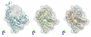
The structures are compared in the figure below. The target map with the initial structure after Situs fitting is in cyan, the best fitted structure after REMD is shown as red spheres, the best fitted structure after targeted MD is in green, the best fitted structure after MD refinement is in orange together with the target structure, again in cyan. The multi-scale protocol facilitated obtaining a structure very close to the target one. Adenylate Kinase shows a relatively easy domain movement and it was used in this tutorial due to its small size that makes the calculations less time-consuming. However, the multi-scale protocol is dedicated mainly for the protein systems with complex domain movements, that are hard to capture using a one-step flexible fitting simulation.
References
[1] M. Kulik et al., Front. Mol. Biosci., 8, 631854 (2021).[2] O. Miyashita et al., J. Comput. Chem., 38, 1447-1461 (2017).
[3] J. Karanicolas and C. Brooks, Prot. Sci., 11, 2351-2361 (2002).
[4] J. Karanicolas and C. Brooks, J. Mol. Biol., 334, 309-325 (2003).
[5] T. Mori et al., Structure, 27, 161-174 (2019).
Written by Marta Kulik@RIKEN Theoretical molecular science laboratory & University of Warsaw
February, 2021
Updated by Cheng Tan@RIKEN
March, 2022