15.1 What is QM/MM?
QM/MM method is a multiscale/multiphysics approach, first proposed in seminal papers by Warshel and Karplus [1] and Warshel and Levitt [2], which treats a chemically important region by the electronic structure theory (QM) and the surrounding environment by a molecular mechanics force field (MM). The method was recently implemented into GENESIS [3,4]. In this section, we give a brief introduction to the theory.
1. MM force field
The potential energy is a pre-requisite to perform molecular simulations. In the MM force field, the potential energy is divided into bonded and non-bonded contribution,
\( \displaystyle V^{MM} = V_{bonded} + V_{non-bonded}. \)
Although the precise functional forms are different in every MM force fields, the former is often represented as a function of bond distances (r), bond angles (\( \theta \)), and torsion angles(\( \phi \)) as,
\( \displaystyle V_{bonded} = \sum_{bond (r)} \frac{k_r}{2} (r – r_0)^2 + \sum_{angle(\theta)} \frac{k_\theta}{2}(\theta – \theta_0)^2 + \sum_{torsion(\phi)} k_\phi[1-\cos(n\phi+\delta)], \)
and the latter is a sum of the Coulomb interaction between atomic charges and the van der Waals interaction,
\( \displaystyle V_{non-bonded} = \sum_{m,m^\prime} \frac{q_m q_{m^\prime}}{|r_m – r_{m^\prime}|} + \sum_{m,{m^\prime}} \epsilon_{m{m^\prime}} \left[ \left( \frac{R^{min}_{m{m^\prime}}}{r_{m{m^\prime}}} \right)^{12} – 2 \left( \frac{R^{min}_{m{m^\prime}}}{r_{m{m^\prime}}} \right)^{6} \right]. \)
The physical simplicity and careful parameterization have led to the enormous success of the MM force field today. However, there are limitations that are evident from its function form: (1) The bond connectivity is pre-defined, so that bond breaking/forming events, i.e., chemical reactions, do not happen during the simulation. (2) The atomic charge is fixed, neglecting the polarization and charge transfer effects. (3) The parameters are usually derived for the electronic ground state, so that the simulation involving electronic excited states is not readily feasible. The motivation of QM/MM method is to overcome the limitations of MM force field.
2. QM/MM potential
In the QM/MM method, the system is spatially divided into QM and MM regions. In the QM region, the motion of electrons is explicitly taken into account based on quantum mechanics. The electronic Schrödindger equation reads in atomic unit,
\( \displaystyle \hat{H}_e = -\frac{1}{2} \sum_i \nabla_i^2 + \sum_{i>i^{\prime}} \frac{1}{|r_i – r_i^{\prime}|} – \sum_{i,a} \frac{Z_a}{|r_i – r_a|} – \sum_{i,m} \frac{q_m}{|r_i – r_m|}, \\ \displaystyle \hat{H}_e |\Psi_e \rangle = E_e |\Psi_e \rangle, \)
where i, a, and m are indices for electrons, nucleus, and MM atoms, respectively. As in the usual electronic structure theory, the first three terms in the Hamiltonian represent the kinetic energy of electrons, the electron-electron repulsion, and the electron-nulceus attraction. The last term represents the Coulomb interaction between the electrons and MM atomic charges, and is unique in the QM/MM method. Note that the interaction is a 1-electron operator, which hardly affects the scaling of QM calculations.
The electronic energy is a function of nuclear and atomic coordinates,
\( \displaystyle E_e = E_e \left( \mathbf{r}_a, \mathbf{r}_m \right). \)
The potential energy of the QM/MM system is then written as,
\( \displaystyle V = V^{QM} \left( \mathbf{r}_a, \mathbf{r}_m \right) + V_{LJ}^{QM/MM} \left( \mathbf{r}_a, \mathbf{r}_m \right) + V^{MM} \left( \mathbf{r}_m \right), \)
where \( V^{QM} \) is the QM energy given as,
\( \displaystyle V^{QM} = E_e \left( \mathbf{r}_a, \mathbf{r}_m \right) + \sum_{a>a^{\prime}}\frac{Z_a Z_{a^\prime}}{|r_a – r_{a^\prime}|} + \sum_{a,m} \frac{Z_a q_m}{|r_a – r_m|}, \)
and \( V^{QM/MM}_{LJ} \) is the Lennard-Jones interaction between QM and MM atoms,
\( \displaystyle V^{QM/MM}_{LJ} = \sum_{a,m} \epsilon_{am} \left[ \left( \frac{R^{min}_{am}}{r_{am}} \right)^{12} – 2 \left( \frac{R^{min}_{am}}{r_{am}} \right)^{6} \right]. \)
The derivatives of the QM/MM potential give the forces acting on the QM and MM atoms,
\( \displaystyle \mathbf{F}_a = -\frac{\partial V}{\partial \mathbf{r}_a} = -\nabla_a V^{QM} – \nabla_a V_{LJ}^{QM/MM}, \\ \displaystyle \mathbf{F}_m = -\frac{\partial V}{\partial \mathbf{r}_m} = -\nabla_m V^{QM} – \nabla_m V_{LJ}^{QM/MM} – \nabla_m V^{MM} \)
Among the QM/MM potential, \( V^{MM} \), \( V_{LJ}^{QM/MM} \), and their derivatives are calculated internally by GENESIS. On the other hand, we expect that \( V^{QM} \) and its derivatives are provided by an external QM program that is capable of solving the electronic Schrödindger equation. Therefore, the QM/MM calculation requires a QM program in addition to GENESIS.
3. Interface with QM programs
GENESIS has a general interface, which makes feasible to easily connect with any QM programs. The structure of the interface is sketched in the figure below,
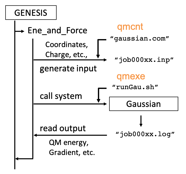
qmcnt and qmexe are the options specified in a [QMMM] section of the control file. qmcnt is a template file to generate input files for the QM program and qmexe is a script file to invoke the QM program.
In the current version, GENESIS is interfaced with
- DFTB+, Version 18, 19, and 20.
- Q-Chem, Version 4.2, 4.3, and 4.4.
- Gaussian, Version 09 and 16.
- TeraChem, Version 1.93P, 1.94V.
- QSimulate
Examples of qmcnt and qmexe files for these programs are found in our github repository.
References
- A. Warshel and M. Karplus, J. Am. Chem. Soc., 94, 5612-5625 (1972).
- A. Warshel and M. Levitt, J. Mol. Biol., 103, 227-249 (1976).
- K. Yagi, K. Yamada, C. Kobayashi, and Y. Sugita, J. Chem. Theory Comput. 15, 1924-1938 (2019).
- K. Yagi, S. Ito, and Y. Sugita, J. Phys. Chem. B 125, 4701-4713 (2021).
Updated by Kiyoshi Yagi@RIKEN Theoretical molecular science laboratory
Feb., 20, 2022
Written by Kiyoshi Yagi@RIKEN Theoretical molecular science laboratory
Dec., 5, 2020