4.2 Statistical analysis of the trajectory data by Awk
Contents
Preparation
Let’s download the tutorial file (tutorial19-4.2.zip).
# Download the tutorial file
$ cd ~/GENESIS_Tutorials-2019/Works
$ mv ~/Downloads/tutorial19-4.2.zip ./
$ unzip tutorial19-4.2.zip

# Clean up the working directory
$ mv tutorial19-4.2.zip ./TRASH

$ cd ./tutorial-4.2
$ ls
Analysis1   Analysis2.1   Analysis2.2
1. Analyze the statistics
In this tutorial, we will learn how to calculate the average, standard deviation, maximum and minimum values of physical quantities obtained by analyzing trajectory data. Some people may want to use “Microsoft Excel” or similar software for this purpose. However, simple statistics can be easily and quickly calculated by executing a single line of command. The following is an example of analyzing the energy trajectory data obtained in Tutorial 3.1 (the header and step 0 lines have been removed beforehand).
# Change directory for statistics analysis
$ cd Analysis1
$ ls
energy.log
1.1 Averaged value
# Compute the averaged value of the 5th column
$ awk '{sum+=$5} END {print sum/NR}' energy.log
-1.51401
1.2 Standard deviation
# Compute the standard deviation of the 5th column
$ awk '{sum+=$5;sum2+=$5*$5} END {print sqrt(sum2/NR-(sum/NR)^2)}' energy.log
2.83058
1.3 Minimum and maximum values
# Compute the minimum value of the 5th column
$ awk 'BEGIN {min= 9999} {if($5<min) min=$5} END {print min}' energy.log
-10.2807

# Alternative command using sort
$ awk '{print $5}' energy.log | sort -g | head -1
-10.2807
# Compute the maximum value of the 5th column
$ awk 'BEGIN {max=-9999} {if(max<$5) max=$5} END {print max}' energy.log
7.3745

# Alternative command using sort
$ awk '{print $5}' energy.log | sort -g | tail -1
7.3745
2. Analyze the histogram
In Section 2, we learn how to analyze histogram or frequency of the data.
2.1 1D-Histogram
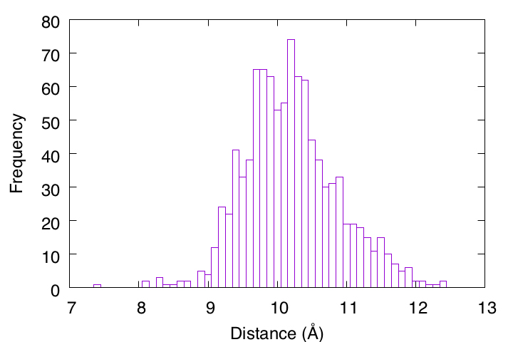
First, we will analyze the distance trajectory data (output.dis) obtained in Tutorial 3.2 and draw a 1D histogram. This directory already contains the analysis program (hist1d.awk), which is written in awk language. In the header part of the program, you can see that the bin size of the histogram (binsizex) and the analysis range (xmin to xmax) are specified. Here, we are analyzing the second column ($2) of output.dis, which is specified in the middle part.
# Change directory for analysis of the 1D histogram
$ cd ../Analysis2.1
$ ls
output.dis  hist1d.awk

# View the program
$ less hist1d.awk
# 1D histogram analysis
#
BEGIN {
xmin = 0.0; xmax = 15.0; binsizex = 0.1;
nx = (xmax - xmin)/binsizex;
for (i=0; i<=nx; i++) freq[i]=0
}
{ i = int(($2 - xmin)/binsizex);
freq[i] = freq[i] + 1 }
END {
for (i=0; i<=nx; i++) {
x0 = xmin + i*binsizex;
print x0, freq[i], freq[i]/NR
}
}
Let’s execute the program for output.dis, where “out” is obtained with the following command.
# Analysis of the 1D histogram
$ awk -f hist1d.awk output.dis > out

# Visualize the results
$ gnuplot
gnuplot> set encoding iso
gnuplot> unset key
gnuplot> set xlabel "Distance (\305)"
gnuplot> set ylabel "Frequency"
gnuplot> plot [7:13][]'out' u 1:2 with boxes
2.2 2D-Histogram
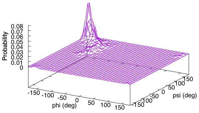
Next, we will analyze the Ramachandran plot data (output.tor) obtained in Tutorial 3.1 to draw a 2-D histogram (or probability distribution). The analysis program (hist2d.awk) is already included in the directory, and it is a 2D extension of the previous 1D program. In the header part of the program, you can see that the bin size of the histogram for each dimension (binsizex, binsizey) and the analysis range (xmin to xmax, ymin to ymax) are specified. We will analyze the second ($2) and third ($3) columns of output.tor as specified in the middle row.
# Change directory for analysis of the 2D histogram
$ cd ../Analysis2.2
$ ls
output.tor  hist2d.awk

$ View the program
$ less hist2d.awk
# 2D histogram analysis
#
BEGIN {
xmin = -180.0; xmax = 180.0; binsizex = 10.0;
ymin = -180.0; ymax = 180.0; binsizey = 10.0;
nx = (xmax - xmin)/binsizex;
ny = (ymax - ymin)/binsizey;
for (i=0; i<=nx; i++) for (j=0; j<=ny; j++) freq[i,j]=0
}
{ i = int(($2 - xmin)/binsizex);
j = int(($3 - ymin)/binsizey);
freq[i,j] = freq[i,j] + 1 }
END {
for (i=0; i<=nx; i++) {
for (j=0; j<=ny; j++) {
x0 = xmin + i*binsizex;
y0 = ymin + j*binsizey;
print x0, y0, freq[i,j], freq[i,j]/NR
}
print " "
}
}
Let’s execute the program for output.tor, where “out” is obtained with the following command.
# Analysis of the 2D probability distribution
$ awk -f hist2d.awk output.tor > out

# Visualize the results
$ gnuplot
gnuplot> unset key
gnuplot> set xlabel "phi (deg)"
gnuplot> set ylabel "psi (deg)"
gnuplot> set zlabel "Probability"
gnuplot> set zlabel rotate by 90
gnuplot> splot [-180:180][-180:180][]'out' u 1:2:4 with lines
Written by Takaharu Mori@RIKEN Theoretical molecular science laboratory
Feb. 24, 2022