16.4 Vibrational analysis of a phosphate ion in solution
Contents
1. Introduction
In this section, we will calculate the infrared (IR) spectrum of a phosphate ion (H2PO4−) in water solution using QM/MM. This system has been studied by QM/MM [1, 2] and ab initio MD [3]. These works have reported strong solvation effects on the IR spectrum, i.e., there is a large spectral shift in the spectrum between the gas-phase and solution due to strong hydrogen bonds (HBs) of H2PO4− and water molecules. The treatment of HB interaction is of essential importance to reproduce the experimental IR spectrum accurately.
Here, we carry out QM/MM calculations, in which the solute is treated by DFT at the level of B3LYP/cc-pVDZ and the water molecules by TIP3P force field. The QM calculations are performed using Gaussian16. The IR spectrum is obtained by solving the vibrational Schrödinger equation (VSE),
\( \displaystyle \left[ -\frac{1}{2} \sum_{i=1}^f \frac{\partial^2}{\partial Q_i^2} + V(\mathbf{Q}) \right]\Psi_n(\mathbf{Q}) = E_n \Psi_n(\mathbf{Q}), \)
where \( f \) is the number of degrees of freedom, \( \mathbf{Q} = (Q_1, Q_2, \cdots, Q_f) \) is the vibrational modes, and \( V(\mathbf{Q}) \) is the potential energy surface (PES). In the harmonic approximation, the PES is truncated at the second-order Taylor expansion around the equilibrium geometry,
\( \displaystyle V(\mathbf{Q}) \simeq V_0 + \sum_{i=1}^f c_{ii} Q_i^2, \)
where the analytical solution to the VSE can be obtained. We also demonstrate anharmonic vibrational calculations, which incorporate the third- and higher-order terms of the PES. The latter is performed by combining GENESIS with SINDO program. SINDO is used to generate the anharmonic potential [4] and to solve the VSE by the second-order vibrational quasi-degenerate perturbation theory (VQDPT2) [5,6].
2. Preparation
Download the tutorial file (tutorial19-16.4.zip or github), unzip it, and proceed to tutorial-16.4. This directory contains nine sub-directories.
$ unzip tutorial19-16.4.zip
$ cd tutorial-16.4
$ ls
0_qmmm_md/  1_setup/    2_minimize/ 3_harmonic/
4_qff/      5_grid/     6_vib/      sindo/       toppar/
0.qmmm_md contains input files to setup H2PO4− in a water box and to perform QM/MM-MD simulations using DFTB3. The simulation can be performed in the same way as in Section 16.2. Although we just leave the input files and don’t go into the details here, interested readers are encouraged to try them out.
1.setup contains the outcome of the QM/MM-MD simulation,
$ ls 1_setup
cmd_100.crd    cmd_100.pdb    cmd_100.psf    qmmm_prod.rst
cmd_100.pdb/psf is H2PO4− in a water sphere of 40 Å diameter obtained from a MD snapshot using qmmm_generator, and qmmm_prod.rst is a restart file of the QM/MM-MD simulation. toppar is already included in the zip file,
$ ls toppar
po4.prm     po4.rtf
po4.rtf/prm contain the topology and parameter of H2PO4− and TIP3P water.
3. Geometry optimization
Let’s proceed to 2_minimize,
$ cd 2_minimize
$ ls
gaussian.com  minimize.gpi  qmmm_min.inp  run.sh   runGau.sh
gaussian.com is a template to generate an input file of Gaussian, and runGau.sh is a script to invoke Gaussian from GENESIS. qmmm_min.inp is a control file of GENESIS, and run.sh is a script to run GENESIS. We will look into these files in the following.
(a) The template file of Gaussian
Important keywords of gaussisan.com are listed below.
%chk=gaussian.chk               (1)
...
scf(conver=8) iop(4/5=100) NoSymm Charge Force Prop=(Field,Read) pop=mk        (2)
...
#coordinate#       (3)
#charge#           (4)
#elec_field#       (5)
(1) The name of a checkpoint file must be “gaussian.chk”. Never remove or change this line.
(2) These are keywords for Gaussian.
scf(conver=8) runs the SCF calculation with a convergence criterion of 10-8 Hartree. The threshold is reduced by 2 upon restart.
iop(4/5=100) is a directive to read molecular orbitals (MO) from a checkpoint file if present.
NoSymm prevents reorientation of axis.
Charge reads MM coordinates and charges.
Force calculates the force in addition to the energy.
Prop=(Field,Read) calculates the electric field at given positions.
pop=mk calculates the ESP charge of QM atoms obtained by fitting the electrostatic potential generated by the electron density to that of atomic charges. Note that this option must be present if macro=YES in [MINIMIZE] (see below).
(3), (4), (5) are replaced by the coordinates of QM atoms, the coordinates and charge of MM atoms, and the coordinates of MM atoms, respectively, at runtime by GENESIS.
See Appendix A for further details on the input options.(b) The script file to run Gaussian
The first part of runGau.sh is shown below. The text in red must be properly set by users,
export g16root=/path/to/gaussian        (1)
export GAUSS_EXEDIR=$g16root/g16
export GAUSS_EXEBIN=$g16root/g16/g16
export PATH=$PATH:$GAUSS_EXEDIR
export LD_LIBRARY_PATH=${GAUSS_EXEDIR}:${LD_LIBRARY_PATH}

# --- Set the path for a scratch folder ---
scratch=/scr/$USER                      (2)
# (optional)
# --- Set a chkpoint file to read initial MOs ---
#initialchk='../path/to/initial.chk'    (3)
(1) Set a path to a folder where Gaussian is installed.
(2) Set a path to a scratch folder. If your machine has a fast, local disk equipped, it is better to use it as a scratch folder. Guassian (and most QM programs) writes a large intermediate file, so that the speed of disk access may significantly affect the performance.
(3) Optionally, set a checkpoint file to read initial MO. (See Section 4)
Note that GENESIS calls the script in the following way,
$ runGau.sh job.com job.log 0
where the first and second arguements are the name of input and output files of Gaussian, respectively, and the third one is the step number in MINIMIZE or MD. It is a good practice to test the script with the above command and see if Gaussian runs properly.
(c) The control file of GENESIS
qmmm_min.inp is similar to the one in Section 6.2 (tutorial-16.2/3_qmmm/qmmm_min.inp), but has different entries in [QMMM] and [MINIMIZE] sections.
[QMMM]
qmtyp              = gaussian            (1)
qmcnt              = gaussian.com        (2)
qmexe              = runGau.sh           (3)
qmatm_select_index = 2                   (4)
...

[SELECTION]
group1  = ...
group2  = sid:PO4                        (5)
(1) qmtyp is set to Gaussian.
(2) (3) qmcnt and qmexe are set to gaussian.com and runGau.sh, respectively.
(4) (5) qmatm_select_index = 2 points to group2 in [SELECTION]. H2PO4− is selected as a QM region.
The [MINIMIZE] section looks like this,
[MINIMIZE]
method              = LBFGS   (1)
nsteps              = 500     # number of steps
eneout_period       = 1       # energy output period
crdout_period       = 5       # coordinates output period
rstout_period       = 1       # restart output period
nbupdate_period     = 1       # non-bonded pair-list update period
macro               = YES     (2)
nsteps_micro        = 100
fixatm_select_index = 1       (3)

[SELECTION]
group1  = not (sid:PO4 around_res: 15.0 or sid:PO4)
(1) LBFGS is an efficient algorithm to energy-minimize the structure, and is suitable for a tight optimization prior to vibrational analyses. SD is not recommended here.
(2) macro = yes invokes a macro/micro-iteration method. In this scheme, the optimization is carried out in two loops. Both QM and MM atoms are relaxed in the outer loop, while only MM atoms are relaxed with QM atoms fixed in the inner loop. During the inner loop, the QM atoms are represented by ESP charges and QM calculations are not required. Thus, it leads to a significant speed up of the calculation.
(3) fixatm_select_index = 1 fix the atoms specified in group1 of [SELECTION]. In this example, water molecules that are distant from H2PO4− by more than 15.0 Å are fixed.
Run the program using run.sh,
$ chmod +x run.sh
$ ./run.sh
The convergence of optimization is checked by the magnitude of root-mean-square gradient (RMSG) and the maximum gradient (MAXG). The tolerance is set to be 0.36 and 0.54 kcal mol-1 Å-1 by default. These values can be changed by tol_rmsg and tol_maxg in the [MINIMIZE] section.
In this example, the convergence will reach in around 50 cycles. The following message appears in the end of the log file when the convergence is reached.
>>>>> STOP: RMSG and MAXG becomes sufficiently small
Let us plot the variation of the potential energy and MAXG as a function of step number.
> grep INFO qmmm_min.out > minimize.log 2>&1
> gnuplot minimize.gpi
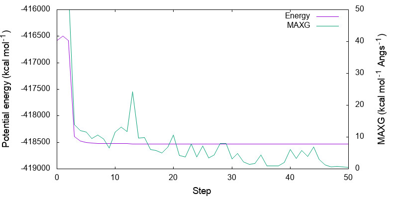
Because the variation in the potential energy is huge in the first few steps, you may adjust the range of y-axis by modifying minimize.gpi,
> vi minimize.gpi
...
set yrange  [-418535:-418500]
...

> gnuplot minimize.gpi
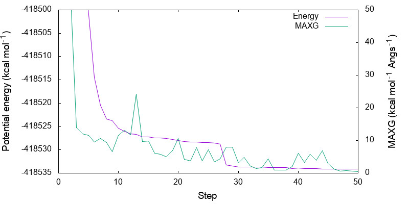
You can see that both energy and MAXG become small along the step. Note that the energy is converged with an accuracy of 1 kcal mol-1 around the 30-th step, while it takes 20 more steps to converge MAXG. A similar behavior is often seen for geometric parameters.
4. Harmonic vibrational analysis
Now, we carry out the harmonic vibrational analysis. In this calculation, the Hessian matrix of a partial system is calculated by numerical differentiations of the gradient. It requires the gradient at 6N + 1 grid points, where N is the number of atoms of the target molecule. The calculation is parallelized over the grid points, i.e., multiple QM calculations run simultaneously for different grid points. Furthermore, we use the molecular orbitals (MOs) obtained at the equilibrium geometry for the initial MOs of SCF calculations at each grid point. The restart of MOs significantly speed up the SCF convergence.
$ cd 3_harmonic
$ ls
gaussian.com   plotIR.gpi   plotIR.sh   qmmm_harm.inp   run.sh   runGau.sh
qmmm_harm.inp is the control file of GENESIS. [INPUT] and [OUTPUT] sections look like this:
[INPUT]
topfile = ../toppar/po4.rtf            # topology file
parfile = ../toppar/po4.prm            # parameter file
psffile = ../1_setup/cmd_100.psf       # protein structure file
pdbfile = ../1_setup/cmd_100.pdb       # PDB file
rstfile = ../2_minimize/qmmm_min.rst   (1)

[OUTPUT]
minfofile = qmmm_harm.minfo            (2)
(1) restarts from the optimized structure obtained in 2_minimize.
(2) minfofile is an output file, where the normal modes and harmonic frequencies are written.
Instead of [MINIMIZE], we now have a new section, [VIBRATION].
[VIBRATION]
runmode             = HARM          (1)
nreplica            = 2             (2)
vibatm_select_index = 3             (3)
output_minfo_atm    = 4             (4)

[SELECTION]
...
group3  = sid:PO4                   (5)
group4  = sid:PO4 around_res:3.0    (6)
(1) sets the calculation to the harmonic analysis.
(2) specifies the number of QM (=MPI) processes to run in parallel.
(3) and (5) set the target molecule of vibrational calculations to H2PO4−.
(4) and (6) set the atoms printed to the minfo file to H2PO4− and water molecules within 3.0 Å of H2PO4−.
gaussian.com is the same as the previous one in 2_minimize. runGau.sh is also the same except that we use the MOs of the last run for the initial MOs,
# --- Set a chkpoint file to read initial MOs ---
initialchk='../2_minimize/qmmm_min.0/gaussian.chk'
In run.sh, we specify 2 MPI processes. Note that the number of MPI processes must be the same or multiples of nreplica in [VIBRATION]. Assuming that we use 1 node with 16-core CPU,
export  QM_NUM_THREADS=8
export OMP_NUM_THREADS=8

# 1) Open MPI
#
mpirun -np 2 --map-by node:pe=${QM_NUM_THREADS} $GENESIS qmmm_harm.inp > qmmm_harm.out 2>&1

# 2) Intel MPI
#
#mpirun -np 2 -ppn 2 $GENESIS qmmm_harm.inp > qmmm_harm.out 2>$1
With this setting, we will have 2 MPI processes running in a node. Let’s run the program,
$ chmod +x run.sh
$ ./run.sh
In the output file (qmmm_harm.out), we can check the atoms selected for vibrational analysis,
Enter vibrational analysis

  Cartesian coordinates of atoms for vib. analysis
     1   1 PO4   1 PO42   P     -5.0216935451    -10.7075582221     -5.3890709445
     2   2 PO4   1 PO42   O1    -5.6128257332    -10.8802681545     -3.8550956045
     3   3 PO4   1 PO42   H1    -5.4714433764    -11.7843520102     -3.5086043226
     4   4 PO4   1 PO42   O2    -5.7403129966     -9.2977042064     -5.7845382483
     5   5 PO4   1 PO42   H2    -6.7222316005     -9.3549834289     -5.7006580436
     6   6 PO4   1 PO42   O3    -3.5100721734    -10.4488167274     -5.4038611074
     7   7 PO4   1 PO42   O4    -5.5363941548    -11.8686855373     -6.2753623567
Then, we see the iteration over grid points,
Generate Hessian matrix by num. diff. of gradients
Loop over atoms
      Done for    0   input       replicaID =     1  energy =       -418534.145104
      Done for   21   O2  +Y      replicaID =     2
      Done for    1   P   +X      replicaID =     1
      Done for   22   O2  +Y      replicaID =     2
      Done for    2   P   +X      replicaID =     1
...
      Done for   42   O4  +Z      replicaID =     2

  RMSD of the gradient at the input geometry =    0.198811D+00 [kcal mol-1 Angs-1]
It is a good practice to make sure that the gradient at the input geometry (= equilibrium geometry) is sufficiently small. You will see a warning message if the gradient is large. In that case, check if the input geometry (rstfile) is correct, if the preceding minimization is converged, and so on. Then, the harmonic frequencies (in cm-1), infrared (IR) intensity (in km mol-1), and normal displacement vectors are printed,
  Harmonic frequencies and normal displacement vectors
          mode             1           2           3           4           5
          omega        123.7917    155.1630    163.7271    194.8849    229.0114
         IR int.         6.4719      5.9877      5.0536      5.2343      3.0750
         1   P    X      0.2251     -0.0904     -0.3468     -0.1093     -0.1671
         1   P    Y      0.0003      0.5412      0.0397     -0.2286      0.0281
         1   P    Z      0.3616      0.0503      0.3070      0.3317     -0.1136
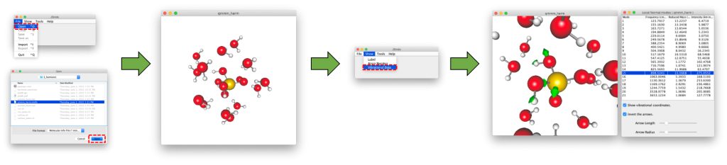
The minfo file (qmmm_harm.minfo) can be visulalized using JSindo. See Appendix C how to download and install the program. JSindo is invoked by the following command (on your local computer)
$ . ../sindo/sindo-4.0/sindovars.sh
$ java JSindo
Then, proceed to File → Open → Choose qmmm_harm.minfo. You will see the molecule show up on the screen. Then, goto Show → Vibrational Data. It will bring up a table of vibrational frequencies. By clicking one of the frequency, the corresponding vibrational mode is depicted in the molecular view.
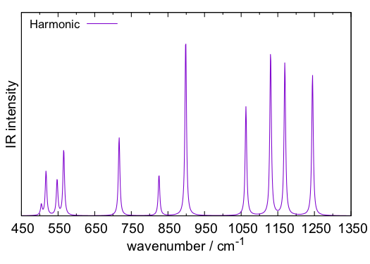
The IR spectrum can be plotted using HarmSpectrum tool in SINDO. plotIR.sh is a script to do this,
$ cat plotIR.sh
#!/bin/bash

. ../sindo/sindo-4.0/sindovars.sh
java HarmSpectrum qmmm_harm.minfo 5 300 1800 1 > harmonic.spectrum
gnuplot plotIR.gpi
The arguments of HarmSpectrum are the name of minfo file, the width of Lorentz function, the range of plot (300 – 1800 cm-1), and the interval of the plot data (1 cm-1). By running the script,
$ chmod +x plotIR.sh
$ ./plotIR.sh
$ ls
plotIR.sh  plotIR.gpi  plotIR.pdf   ...
we obtain a plot of the IR spectrum, plotIR.pdf, which looks like this,
5. Anharmonic vibrational calculations
We now perform anharmonic vibrational analysis. Since this section requires SINDO program, first see Appendix C and setup the program if you haven’t done it yet.
(a) Generation of the anharmonic PES
We first generate the anharmonic PES. The functional form of the PES is a combination of the quartic force field (QFF) and a one-dimensional (1D) grid PES. QFF reads,
\( \displaystyle V^{\mathrm{QFF}}(\mathbf{Q}) = V_0 + \sum_{i=1}^f c_{ii} Q_i^2 + \sum_{i, j, k}^f c_{ijk} Q_iQ_jQ_k + \sum_{i, j, k,l}^f c_{ijkl} Q_iQ_jQ_kQ_l, \)
and the 1D-grid PES is,
\( \displaystyle V^{\mathrm{1D-grid}} (\mathbf{Q}) = \sum_{i=1}^f V_i(Q_i) \)
where \( V_i(Q_i) \) is a potential energy function along \( Q_i \) in a descritized, grid representation.
Proceed to 4_qff,
$ cd 4_qff
$ ls
gaussian.com  makePES.xml   makePES1.sh*  makePES2.sh*  qmmm_qff.inp  run.sh*       runGau.sh*
makePES1.sh is a script to invoke RunMakePES tool of SINDO.
$ cat makePES1.sh
#!/bin/bash

. ../sindo/sindo-4.0/sindovars.sh
java RunMakePES -f makePES.xml > makePES.out1  2>&1
makePES.xml is the input file of RunMakePES to generate QFF. We don’t go into detail of this file here, but interested readers are referred to the Users’ guide ot SINDO. Run the script by typing,
$ chmod +x makePES1.sh
$ ./makePES1.sh
$ ls
gaussian.com  makePES.xml   makePES2.sh*  qmmm_qff.inp  runGau.sh*
makePES.out1  makePES1.sh*  makeQFF.xyz   run.sh*
The command creates makeQFF.xyz. This file contains coordinates of the target molecule, i.e., H2PO4–, at grid points where the energy and gradient are needed.
qmmm_qff.inp is the control file of GENESIS, which is the same as qmmm_harm.inp except for the [VIBRATION] section,
[VIBRATION]
runmode             = QFF           (1)
nreplica            = 2
vibatm_select_index = 3
gridfile            = makeQFF.xyz   (2)
minfo_folder        = minfo.files   (3)
(1) sets the calculation to QFF generation.
(2) specifies the file that contains the coordinates of grid points.
(3) specifies the directory where intermediate minfo files are stored.
run.sh is a script to run GENESIS, which is the same as before. Now, let’s run the job,
$ chmod +x run.sh
$ ./run.sh
We can check the iteration over the grid points in the output, qmmm_qff.out,
 Compute energy at grid points: minfo files created in [ minfo.files ]
      Done for             mkqff-eq :    replicaID =     2
      Done for             mkqff8-0 :    replicaID =     1
      Done for             mkqff8-2 :    replicaID =     1
      Done for             mkqff8-1 :    replicaID =     2
...
and the information at each grid point is written to minfo.files/mkqff-*.minfo.
$ ls minfo.files
mkqff10-0.minfo     mkqff14_8-0.minfo   mkqff17_13-3.minfo  mkqff19_15-3.minfo
mkqff10-1.minfo     mkqff14_8-1.minfo   mkqff17_14-0.minfo  mkqff19_16-0.minfo
...
When the GENESIS job is done, we invoke the RunMakePES tool again,
$ cat makePES2.sh
#!/bin/bash

. ../sindo/sindo-4.0/sindovars.sh
java RunMakePES -f makePES.xml >& makePES.out2

$ chmod +x makePES2.sh
$ ./makePES2.sh
$ ls
gaussian.com   makePES.xml    makePES.out1  makePES.out2  makeQFF.xyz_0
minfo.files/   prop_no_1.mop  qmmm_qff.0/   qmmm_qff.1/   qmmm_qff.inp
qmmm_qff.out   run.sh         runGau.sh
Although the command and the input file for RunMakePES are the same as before, the program retrieves the information from minfo.files/*.minfo, and prints the QFF coefficients to prop_no_1.mop.
The grid PES can be generated in the same manner. Proceed to 5_grid,
$ cd 5_grid
$ ls
gaussian_ene.com  makePES1.sh      qmmm_grid.inp     runGau.sh
makePES.xml       makePES2.sh      run.sh
qmmm_grid.inp is an input of GENESIS, in which the [VIBRATION] section looks like this,
[VIBRATION]
runmode             = GRID                (1)
nreplica            = 2
vibatm_select_index = 3
gridfile            = makeGrid.xyz        (2)
datafile            = makeGrid.dat        (3)
(1) sets the calculation to grid PES generation.
(2) specifies the file that contains the coordinates of grid points.
(3) specifies the file where the energy and dipole moment are written.
In the grid PES generation, we calculate the energy and dipole moment, but don’t need the gradient. Therefore, the template of Gaussian, gaussian_ene.com, doesn’t have the “force” keyword.
#P B3LYP/cc-pVDZ EmpiricalDispersion=GD3
scf(conver=8) iop(4/5=100) NoSymm
Charge  (Force is removed)
Now, let’s run the job.
$ chmod +x run.sh makePES1.sh makePES2.sh
$ ./makePES1.sh
$ ./run.sh
$ ./makePES2.sh
The first command (makePES1.sh) writes the coordinates of grid points to makeGrid.xyz, and the second command (run.sh) invokes GENESIS. We can check the iteration over the grid points in the output, qmmm_grid.out,
 Compute energy at grid points: data written to [ makeGrid.dat ]
      Done for          mkg-q9-11-0 :    replicaID =     1
      Done for               mkg-eq :    replicaID =     2
      Done for          mkg-q9-11-1 :    replicaID =     2...
and the energy and dipole is written to makeGrid.dat.
$ ls minfo.files
mkg-q9-11-0,   -666.961159903,  7.591214970E+00, 2.097339590E+01, 1.154947680E+01
mkg-q9-11-2,   -666.971926490,  7.601926380E+00, 2.088108250E+01, 1.158874200E+01
mkg-q9-11-4,   -666.976106344,  7.612145000E+00, 2.080164720E+01, 1.161928860E+01
...
The last command (makePES2.sh) creates the grid PES and dipole moment surface (DMS) and stores the information to *.pot and *.dipole, respectively.
$ ls *pot
eq.pot	 q11.pot  q13.pot  q15.pot  q17.pot  q19.pot  q21.pot
q10.pot  q12.pot  q14.pot  q16.pot  q18.pot  q20.pot  q9.pot
$ ls *dipole
eq.dipole   q12.dipole	q15.dipole  q18.dipole	q21.dipole
q10.dipole  q13.dipole	q16.dipole  q19.dipole	q9.dipole
q11.dipole  q14.dipole	q17.dipole  q20.dipole
(b) VQDPT2 calculations
Finally, we carry out VQDPT2 calculations and obtain the anharmonic spectrum. The PES is a composite of QFF and 1D-grid PES,
\( \displaystyle V(\mathbf{Q}) = V^{\mathrm{QFF’}}(\mathbf{Q}) + V^{\mathrm{1D-grid}} (\mathbf{Q}), \)
where \( V^{\mathrm{QFF’}} \) is a QFF without the 1-mode terms,
\( \displaystyle V^{\mathrm{QFF’}}(\mathbf{Q}) = V^{\mathrm{QFF}} – \sum_{i=1}^f [ c_{ii} Q_i^2 + c_{iii} Q_i^3 + c_{iiii} Q_i^4]. \)
Proceed to 6_vib,
$ cd 6_vib
$ ls
plotIR.gpi  run.sh     vqdpt2.inp
run.sh is a script to set the comosite PES and to run VQDPT2. The first part of the script looks like this,
export POTDIR=./pes
if [ -e ${POTDIR} ]; then
  rm -r ${POTDIR}
fi
mkdir ${POTDIR}
cp ../4_qff/prop_no_1.mop ${POTDIR}
cp ../5_grid/*.pot        ${POTDIR}
cp ../5_grid/*.dipole     ${POTDIR}
The information of the PES in 4_qff and 5_grid is gathered to $POTDIR (pes). The composit PES above is specified in this way, becuase the grid PES takes higher priority than QFF. vqdpt2.inp is the input file to carry out VQDPT2 calculations. See SINDO website for the details about the input file.
Let’s run the program,
sindo < vqdpt2.inp > vqdpt2.out 2>&1

gnuplot plotIR.gpi
sindo creates, vqdpt-IR.spectrum, and gnuplot plots the resulting spectrum, which looks like this.
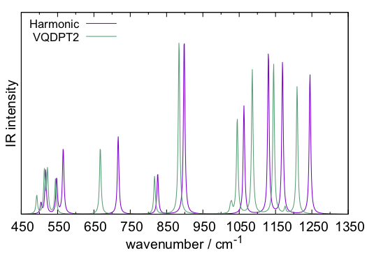
It would be interesting to compare the result with Fig. 4 (d) (e) of Ref. [1]. Although the overall trends are similar, there are some notable differences. One of the reasons is the size of the QM region (and also due to the difference in the basis sets, cc-pVDZ vs cc-pVTZ). In Ref. [1], the water molecules around H2PO4– were also included in the QM region. Such a calculation can be done by setting,
group2 = sid:PO4 around_res: 3.0 or sid:PO4
in the input files of GENESIS. Ref [1] shows the IR spectrum of H2PO4– in the gas phase, i.e., without water molecules, in Fig. 4 (f). A significant change between the gas-phase and solution is noteworthy.
References
[1] K. Yagi, K. Yamada, C. Kobayashi, and Y. Sugita, J. Chem. Theory Comput. 15, 1924-1938 (2019).[2] M. Klaḧn,G. Mathias, C. Kötting,M. Nonella,J. Schlitter, K. Gerwert, and P. Tavan, J. Phys. Chem. A 108, 6186−6194 (2004).
[3] J. VandeVondele, P. Troster, P. Tavan, and G. Mathias, J. Phys. Chem. A 116, 2466−2474 (2012).
[4] K. Yagi, S. Hirata, and K. Hirao, Theor. Chem. Acc. 118, 681-691 (2007).
[5] K. Yagi, S. Hirata, and K. Hirao, Phys. Chem. Chem. Phys. 10, 1781-1788 (2008).
[6] K. Yagi and H. Otaki, J. Chem. Phys. 140, 084113 (2014).
Appendix A. The template input file for Gaussian (gaussian.com)
The template file for Gaussian is the following.
%chk=gaussian.chk                         .... (1)
%NProcShared=8                            .... (2)
%mem=1gb                                  .... (3)
#P b3lyp/cc-pVDZ EmpiricalDispersion=GD3  .... (4)
scf(conver=8) iop(4/5=100) NoSymm Charge  .... (5)
Force Prop=(Field,Read) pop=mk            .... (6)
                                          .... (7)
Gaussian run for QMMM in genesis          .... (8)
                                          .... (9)
-1 1                                      .... (10)
#coordinate#                              .... (11)
#charge#                                  .... (12)
#elec_field#                              .... (13)
(1) specifies the name of a check point file. Don’t change this line unless you are sure!
(2) specifies the number of CPU threads. This line is overwritten to match $QM_NUM_THREADS by runGau.sh (see below).
(3) specifies the amount of memory used by Gaussian. “1gb” means 1 giga-byte. We can also use “mb” for mega-byte. That is, “1000mb” is a synonym of “1gb”. Note that the memory here is only for one Gaussian job. Don’t forget to leave some room for GENESIS. Also, pay attention to the number of QM jobs that runs in a node. The maximum amount of memory specified here would be,
maxMemory = (mem_of_system – mem_for_OS) / (num_of_proc_per_node) – mem_for_GENESIS
(4) – (6): These are options to control QM calculations in Gaussian. Visit the Gaussian website for further details.
b3lyp/cc-pVDZ uses B3LYP functions for DFT and cc-pVDZ for the basis sets
EmpiricalDispersion=GD3 uses D3 dispersion correction
scf(conver=8) sets SCF convergence to 10-8 Hartree.
iop(4/5=100) restarts SCF if the previous MO is present in a checkpoint file (=gaussian.chk)
Nosymm keeps the XYZ orientation of a system
Charge sets MM point charges in QM calculations
Force calculates the gradient of the energy
Prop=(field, read) calculates the electric field applied to MM point charges
pop=mk calculates ESP charges for QM atoms. This is required when macro = yes in [MINIMIZE].
(7) a blank line to set the end of options.
(8) a title line. This can be anything.
(9) a blank line to set the end of a title.
(10) specifies charge and spin multiplicity. Note that the former is the charge of a QM subsystem, not of the whole system. Multiplicity is 2s+1, where s is the spin of a QM subsystem.
(11)-(13) These directives are replaced with the coordinates of QM atoms and MM atoms.
Appendix B. The script to run Gaussian (runGau.sh)
#!/bin/bash
# -----------------------------------------------
# Settings for Gaussian16
#
# --- Set the path for Gaussian ---
export g16root=/usr/local/gaussian      ... (1)
export GAUSS_EXEDIR=$g16root/g16
export GAUSS_EXEBIN=$g16root/g16/g16
export PATH=$PATH:$GAUSS_EXEDIR
export LD_LIBRARY_PATH=${GAUSS_EXEDIR}:${LD_LIBRARY_PATH}

# --- Set the path for a scratch folder ---
scratch=./    ... (2)

# (optional)
# --- Set a chkpoint file to read initial MOs ---
#initialchk='../initial.chk'  ... (3)

QMINP=$1 ...(4)
QMOUT=$2
NSTEP=$3
MOL=${QMINP%.*}

# Initial MO
if [ $NSTEP -eq 0 ] && [ -n "${initialchk}" ] && [ -e ${initialchk} ]; then
   cp ${initialchk} gaussian.chk  ... (5)
fi

# Scratch folder settings
export GAUSS_SCRDIR=$scratch/$(mktemp -u $MOL.XXXX)  ... (6)
mkdir -p ${GAUSS_SCRDIR}

# SMP parallel setting
if [ -z "$QM_NUM_THREADS" ] && [ "${QM_NUM_THREADS:-A}" = "${QM_NUM_THREADS-A}" ]; then
    QM_NUM_THREADS=$OMP_NUM_THREADS  ... (7)
fi
TMP=$(mktemp tmp.XXXX)
echo "%NprocShared=${QM_NUM_THREADS}" >> $TMP
grep -v -i nproc $QMINP >> $TMP ... (8)
mv $TMP $QMINP

# Now exe g16 and create a formatted chk file
(time $GAUSS_EXEBIN < $QMINP) > ${QMOUT} 2>&1      ... (9)
formchk gaussian.chk gaussian.Fchk >& /dev/null

# Remove unnecessary folder
rm -rf ${GAUSS_SCRDIR}   ... (11)
(1) sets the path for Gaussian.
(2) sets the path for scratch files.
(3) modify to use existing check point file for restarting SCF.
(4) sets the input arguments to variables.
(5) copy the saved check point file, which contains the initial MO, to gaussian.chk. Note that this line is executed only for the first step ($NSTEP == 0).
(6) sets $GAUSS_SCRDIR to a temporary folder in $scratch. Gaussian uses this variable for a scratch folder.
(7) checks whether or not $QM_NUM_THREADS is set. If not, it defaults to $OMP_NUM_THREADS.
(8) modifies $QMINP so that %NprocShared equals to $QM_NUM_THREADS.
(9) executes Gaussian, and then generates a formatted checkpoint file (gaussian.Fchk). GENESIS retrieves the QM energy, gradient, and so on, from the log file ($QMOUT) and Fchk file.
(10) removes $GAUSS_SCRDIR. One may add other post processes here, for example, extracting quantities written in the log files. Note that $QMINP, $QMOUT, gaussian.Fchk are removed by GENESIS after reading the QM information if mod(NSTEP/qmsave_period) != 0.
Appendix C. How to download and compile SINDO
The script files to download and compile SINDO are prepared in sindo directory,
$ ls
0_qmmm_md/  1_setup/    2_minimize/ 3_harmonic/
4_qff/      5_grid/     6_vib/      sindo/       toppar/
$ cd sindo
$ ls
comp_sindo.sh     download_sindo.sh
The script, download_sindo.sh, downloads a zip file of the program, unzip it, and creats a file to set up variables (sindo-4.0/sindovars.sh). You’re done if you just want to use JSindo. The following command should work,
$ . sindo-4.0/sindovars.sh
$ java JSindo
If you want to perform the anharmonic calculation, you need to compile the program. Fortran compiler (either intel or gfortran) and blas/lapack libraries are required. Run comp_sindo.sh,
$ ./comp_sindo.sh
///  Welcome to SINDO  ///

...
Select the compiler [ gfortran/gfortranI8 ]
Default=gfortranI8 :  (Just press Enter)
The compiler is automatically detected and you will be asked for the choice. If the default is OK, just press Enter. If you have Intel MKL, the link command is automatically set. In this case, you only need to press Enter again. If you need to (or want to) manually set the BLAS/LAPACK path, it will be like this,
Provide the path for BLAS and LAPACK libraries:
example) -L/usr/local/lib -llapack -lblas
-L /path/to/lapack-3.x.x -l lapack -l blas
In this example, lapack-3.x.x is a directory where liblapack.a and libblas.a are located. Then, the script will compile the program and setup everything. Try the following command,
$ . sindo-4.0/sindovars.sh
$ sindo
 -------------------------------------------------------

    ***   WELCOME TO SINDO PROGRAM
     ***                (  VERSION 4.0 0602  )
...
(press Ctrl-c to quit)
If you see the welcome message, you’re all set! If not, and you encounter any problem, consult the website of SINDO, where further information is available.
by Kiyoshi Yagi@RIKEN Theoretical molecular science laboratory
Jul., 6, 2022