14.1 Replica path sampling of alanine-tripeptide in water
Files for this tutorial (tutorial-14.1.tar)
Contents
- 1. System setup
- 2. Energy minimization and pre-equilibration
- 3. Generating an initial pathway (Steered MD)
- 4. Preparing inputs for replica path sampling (rpath_generator)
- 5. Equilibration along the initial pathway
- 6. Replica path sampling
- 7. Umbrella sampling along the minimum free energy path
- 8. MBAR analysis of the free energy profile along the pathway
GENESIS 1.4 or later is required for this tutorial.
The replica path sampling method (also known as the string method) is a powerful approach to study conformational changes between two different structures of a biomolecule. The method efficiently finds the physically most probable pathway connecting two structures very efficiently, thus enabling us to characterize the molecular mechanism of the conformational change. In the replica path sampling method, a pathway for the conformational change is represented by discrete points (called images) in the collective variable space. Then, a conventional MD simulation is performed around each image to find lower free energy regions while updating images repeatedly to converge to the minimum free energy path.
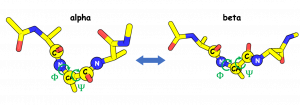
In this tutorial, we explain how to use the replica path sampling method to investigate the conformational change of a small peptide (alanine tripeptide) in water. Alanine tripeptide undergoes a conformational change from an alpha-helix state to a beta-sheet state. Since this process is well characterized by two dihedral angles, Φ and Ψ, we will search for the most probable pathway (called the minimum free energy path) in the subspace spanned by these two collective variables. Please note that it may take around a day or longer to finish all simulations in this tutorial with a single-node machine. We recommend using multiple computation nodes, GPU cluster is the best choice.
All the necessary files for this tutorial can be found in the compressed tar file given above. Unpacking the file creates multiple directories inside tutorial-14.1/. Since the system is identical to the one used in tutorial-3.2, we skip the step of system setup.
1. System setup
In this step, we will prepare a system solvated in a water box. To set up the system, please follow the steps in tutorial-3.2 (“1. Setup”). Copy the output file “wbox.psf” from “tutorial-3.2/1_setup” into the “1_setup” directory of the current tutorial. We also need to make a symbolic link to the CHARMM toppar directory by executing the following command (see Tutorial 2.1):
# Make symbolic link to the CHARMM toppar directory
$ ln -s ../../Others/CHARMM/toppar ./
$ ls
1_setup 2_minim_equil 3_steered_md 4_rpath_generator
5_rpath_equil 6_rpath_prod 7_umbrella 8_mbar toppar

# Copy the psf file in tutorial-3.2 to "1_setup" directory
$ cd 1_setup
$ cp ../tutorial-3.2/1_setup/wbox.psf .
Or you can copy the CHARMM toppar directory to the current tutorial directly. Please note that, we provide an executable script file for every step in this tutorial (“run.sh” in each directory). You can finish each step just by executing the script file (“./run.sh”) in the corresponding directory.
In the “1_setup” directory, we provide two pdb files: “start.pdb” and “end.pdb”, which correspond to the alpha-helix structure and beta-sheet structure of alanine tripeptide respectively. The file “start.pdb”, as the name suggests, is the initial structure of the simulation. While the file “end.pdb” is used as the reference file for the steered MD representing the target states.
2. Energy minimization and pre-equilibration
Next, we will perform minimization and equilibration steps. The general scheme is similar to that shown in tutorial-3.2. Here we only show the sequence of commands for performing the steps.
# Change directory
$ cd 2_minim_equil/

# Run minimization
$ mpirun -np 8 /home/usr/GENESIS/bin/spdyn run_1.inp | tee run_1.log

# Run first-step NVT equilibration
$ mpirun -np 8 /home/usr/GENESIS/bin/spdyn run_2.inp | tee run_2.log

# Run second-step NPT equilibration
$ mpirun -np 8 /home/usr/GENESIS/bin/spdyn run_3.inp | tee run_3.log
3. Generating an initial pathway (Steered MD)
To run replica path sampling, first, we need to generate an initial pathway connecting the start (alpha-helix) and end (beta-sheet) structures. Several methods can be applied to obtain this initial pathway, such as steered/targeted MD simulation and morphing, among others. Here, starting from the alpha-helix structure, we use steered MD simulation to artificially pull the structure toward the beta-sheet structure by imposing a restraint on the RMSD (Root Mean Squared Deviation) variable.
It is noted that, in the case of alanine tripeptide, the result of the steered MD simulation is very sensitive to factors such as the random seed, compiler, and hardware, therefore it is difficult to reproduce the result below (this is due to subtle fluctuations of atoms, periodicity in the torsion space, low free energy barriers, and so on).
The following command executes the simulation:
# Change directory
$ cd 3_steered_md/

# Run steered MD
$ mpirun -np 8 /home/usr/GENESIS/bin/spdyn run.inp | tee run.log
Also, you can run the steered MD by executing the bash script that we provide(“./run.sh”).
The content of run.inp is shown below. Important keywords=values are indicated by red. In the steered MD simulation, reffile is required to provide the structural information of the target state. In this case, we specify reffile=../1_setup/end.pdb which represents the structure of the beta-sheet state. The steered MD scheme is turned on by steered_MD=YES. initial_rmsd is the initial RMSD value for restraint (usually RMSD value of the initial structure from the target is specified). final_rmsd should be close to zero (exact zero might cause a crash in some cases). Fitting of the structure (to reffile) is required for RMSD calculation in order to remove the contributions from global translation and rotations. Thus, fitting_method=TR+ROT (removing TRanslation and ROTation) is specified here.
[INPUT]
topfile          = ../toppar/top_all36_prot.rtf      # topology file
parfile          = ../toppar/par_all36_prot.prm      # parameter file
strfile          = ../toppar/toppar_water_ions.str   # stream file
psffile          = ../1_setup/wbox.psf                # protein structure file
pdbfile          = ../1_setup/start.pdb               # PDB file
reffile          = ../1_setup/end.pdb                 # PDB file for restraints
rstfile          = ../2_minim_equil/eq2.rst           # restart file

[OUTPUT]
rstfile          = run.rst  # restart file
dcdfile          = run.dcd  # dcd trajectory file
dcdvelfile       = run.dvl  # dcd velocity file

[ENERGY]
forcefield       = CHARMM # CHARMM force field
electrostatic    = PME    # Particle Mesh Ewald method
switchdist       = 10.0   # switch distance
cutoffdist       = 12.0   # cutoff distance
pairlistdist     = 13.5   # pair-list distance
vdw_force_switch = YES    # force switch option for van der Waals
pme_nspline      = 4      # order of B-spline in PME
pme_max_spacing  = 1.2    # max grid spacing

[DYNAMICS]
integrator       = LEAP   # leapfrog Verlet integrator
nsteps           = 500    # number of MD steps
timestep         = 0.002  # timestep (ps)
eneout_period    = 2      # energy output period
crdout_period    = 2      # coordinates output period
velout_period    = 2
rstout_period    = 500    # restart output period
nbupdate_period  = 2      # nonbond update period
steered_md       = YES
initial_rmsd     = 3.0    # initial rmsd from reffile
final_rmsd       = 0.01   # final rmsd from reffile
iseed            = 1228373

[CONSTRAINTS]
rigid_bond       = YES      # constraints all bonds involving hydroge

[ENSEMBLE]
ensemble         = NPT      # NPT ensemble
tpcontrol        = LANGEVIN # thermostat and barostat
temperature      = 300.00   # initial and target temperature (K)
pressure         = 1.0      # initial and target pressure (atm)
isotropy         = ISO      # isotropic pressure couplin

[BOUNDARY]
type             = PBC      # periodic boundary condition

[SELECTION]
group1           = rno:1-3 and heavy

[RESTRAINTS]
nfunctions       = 1         # number of restraint functions
function1        = RMSD      # RMSD restraint
reference1       = 3.0       # reference value of a restraint function
constant1        = 1000.0    # force constant of a restraint function
select_index1    = 1

[FITTING]
fitting_method   = TR+ROT    # remove translational and rotational motion
fitting_atom     = 1
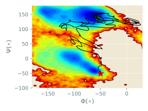
In the figure below, the trajectory of the steered MD simulation (black line) is plotted in the collective variable space (Φ and Ψ). The free energy surface, evaluated from very long brute-force simulations, is drawn for reference. Although the peptide successfully shifts from the initial alpha-helix structure (red star) to the final beta-sheet structure (green star), there are large fluctuations in the trajectory.
4. Preparing inputs for replica path sampling (rpath_generator)
In this step, we generate input files for replica path sampling from the trajectory of the steered MD simulation using the rpath_generator tool in GENESIS. This tool discretizes the initial pathway obtained from the previous step into a predetermined number of images, outputs the coordinates of these images, and restart files for atomistic simulations. First, the trj_analysis tool is used for projecting the steered MD trajectory onto the collective variables space. Then, using the rpath_generator tool, trajectory snapshots are clustered, and coordinates of images are set in an equidistant manner so that the distances between adjacent images are the same. Then, the snapshot most similar (with the collective variable most similar) to the image is extracted for each image. Finally, restart files containing the all-atom coordinates, as well as the corresponding image coordinates are written.
The following commands execute trj_analysis and rpath_generator.
# Change directory
$ cd 4_rpath_generator/

# Project the steered MD trajectory onto the collective variables space
$ /home/usr/GENESIS/bin/trj_analysis trj_analysis.inp

# Generate input files for rpath sampling simulation
$ /home/usr/GENESIS/bin/rpath_generator rpath_generator.inp | tee rpath_generator.log
The content of rpath_generator.inp is shown below. cvfile is a trajectory file projected on the collective variable space (generated by trj_analysis). dcdfile and dcdvelfile are trajectory files of coordinates and velocities of the steered MD simulation, respectively. Note that outputting a velocity file in steered MD is recommended since it allows rpath_generator to generate better restart files. The number of images is specified by nreplica=16. Curly brackets {} in the [OUTPUT] section are replaced with image indices 1,…,16. iseed is used for embedding different seeds for restart files. iter_reparam is a smoothing parameter for defining image coordinates (iter_reparam=10 is recommended).
After running the commands, 16 restart files (1.rst, …, 16.rst) and 16 pdb files (1.pdb, …, 16.pdb) are created. Restart files contain atomistic coordinates as well as coordinates of the corresponding images. PDB files contain only atomistic coordinates.
[INPUT]
cvfile       = tmd.tor
pdbfile      = ../1_setup/start.pdb
dcdfile      = ../3_steered_md/run.dcd
dcdvelfile   = ../3_steered_md/run.dvl

[OUTPUT]
rstfile      = {}.rst  # restart files
pdbfile      = {}.pdb  # pdb files

[RPATH]
nreplica     = 16      # number of replicas
iseed        = 67755
iter_reparam = 10
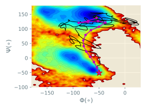
In the figure below, the images (purple circles) generated by rpath_generator are depicted in the collective variable space (Φ and Ψ). It can be seen that the images are located in an equidistant manner in this 2D space.
5. Equilibration along the initial pathway
In this step, we perform a two-step equilibration using 16 replicas (corresponding to 16 images) in order to relax the all-atom structures, while imposing weak and strong restraints on the collective variables (Φ and Ψ) for each replica with respect to its image.
# Change diretory
$ cd 5_rpath_equil/

# Run first-step equilibration with weak restraint
$ mpirun -np 16 /home/usr/GENESIS/bin/spdyn run_1.inp | tee run_1.log

# Run second-step equilibration with strong restraint
$ mpirun -np 16 /home/usr/GENESIS/bin/spdyn run_2.inp | tee run_2.log
The content of run_1.inp is shown below. nreplica=16 in [RPATH] specifies that we perform a simulation of 16 replicas. rpath_period=0 means that references of restraints (image coordinates) do not move during the simulation. Force constants for the restraints are specified in the lists given by constants[1] and constants[2] (for Φ and Ψ, respectively) in [RESTRAINTS]. The first value in each list specifies the force constant of the 1st replica (image), and the 2nd value is the force constant of the 2nd replica, and so on. The weak restraints (constant[12]=1.0 kcal/mol/rad2) applied in the first step of the equilibration were used in order to relax the system. Then, a strong force constant (constant[12]=100.0 kcal/mol/rad2), as recommended for replica path sampling is used in the second equilibration step. Reference values for the restraints are specified by reference[12]. Values were set to 0.0 because GENESIS can automatically replace these values with the coordinates of images embedded in the restart files (generated by rpath_generator).
[INPUT]
topfile          = ../toppar/top_all36_prot.rtf
parfile          = ../toppar/par_all36_prot.prm
strfile          = ../toppar/toppar_water_ions.str
psffile          = ../1_setup/wbox.psf
pdbfile          = ../1_setup/start.pdb
reffile          = ../4_rpath_generator/{}.pdb
rstfile          = ../4_rpath_generator/{}.rst

[OUTPUT]
logfile          = eq1.{}.log      # log file of each replica
dcdfile          = eq1.{}.dcd
rstfile          = eq1.{}.rst
rpathfile        = eq1.{}.rpath

[ENERGY]
forcefield       = CHARMM
electrostatic    = PME
switchdist       = 10.0
cutoffdist       = 12.0
pairlistdist     = 13.5
vdw_force_switch = YES
pme_nspline      = 4
pme_max_spacing  = 1.2
contact_check    = YES

[DYNAMICS]
integrator       = VVER
nsteps           = 50000
timestep         = 0.002
eneout_period    = 1000
crdout_period    = 1000
rstout_period    = 1000
nbupdate_period  = 10

[ENSEMBLE]
ensemble         = NPT
tpcontrol        = BUSSI
temperature      = 300.0
pressure         = 1.0
isotropy         = ISO

[CONSTRAINTS]
rigid_bond       = YES

[BOUNDARY]
type             = PBC

[RPATH]
nreplica         = 16     # number of replicas
rpath_period     = 0      # no update of the image coordinates
rest_function    = 1 2    # index of the restraint function to be used
fix_terminal     = YES    # two terminal images are always fixed

[SELECTION]
group1           = ai:15
group2           = ai:17
group3           = ai:19
group4           = ai:25
group5           = ai:27

[RESTRAINTS]
nfunctions       = 2      # number of restraint functions

function1        = DIHED  # dihedral restraint
constant1        = 1.0 1.0 1.0 1.0 1.0 1.0 1.0 1.0 \
                   1.0 1.0 1.0 1.0 1.0 1.0 1.0 1.0
reference1       = 0.0 0.0 0.0 0.0 0.0 0.0 0.0 0.0 \
                   0.0 0.0 0.0 0.0 0.0 0.0 0.0 0.0
select_index1    = 1 2 3 4     # PHI

function2        = DIHED  # dihedral restraint
constant2        = 1.0 1.0 1.0 1.0 1.0 1.0 1.0 1.0 \
                   1.0 1.0 1.0 1.0 1.0 1.0 1.0 1.0
reference2       = 0.0 0.0 0.0 0.0 0.0 0.0 0.0 0.0 \
                   0.0 0.0 0.0 0.0 0.0 0.0 0.0 0.0
select_index2    = 2 3 4 5     # PSI
6. Replica path sampling
Next, we perform the replica path sampling simulation.
# Change diretory
$ cd 6_rpath_prod/

# Run replica path sampling simulation
$ mpirun -np 16 /home/usr/GENESIS/bin/spdyn run.inp | tee run.log
The content of run.inp is shown below. rpath_period in the [RPATH] specifies the duration of the time window during which the mean force is evaluated (by time-averaging). Here, the image coordinates are updated according to the estimated mean forces every rpath_period=1000 steps (corresponding to 2 ps). Typically 500-5000 steps are recommended for moderate-size biomolecules. delta in [RPATH] is the size of the image update. Using a delta value too large will cause the structure to become unstable, while a small value will result in slow convergence of the pathway. Here too, the reference values reference[12] for the restraints (the initial coordinates of images) are automatically replaced with those embedded in the restart files. The output trajectory files of the image coordinates are specified by rpathfile={}.rpath in [OUTPUT].
[INPUT]
topfile          = ../toppar/top_all36_prot.rtf
parfile          = ../toppar/par_all36_prot.prm
strfile          = ../toppar/toppar_water_ions.str
psffile          = ../1_setup/wbox.psf
pdbfile          = ../1_setup/start.pdb
rstfile          = ../5_rpath_equil/eq2.{}.rst

[OUTPUT]
logfile          = rp.{}.log
dcdfile          = rp.{}.dcd
rstfile          = rp.{}.rst
rpathfile        = rp.{}.rpath     # rpath files containing the image coordinates.

[ENERGY]
forcefield       = CHARMM
electrostatic    = PME
switchdist       = 10.0
cutoffdist       = 12.0
pairlistdist     = 13.5
vdw_force_switch = YES
pme_nspline      = 4
pme_max_spacing  = 1.2

[DYNAMICS]
integrator       = VVER
nsteps           = 100000
timestep         = 0.002
eneout_period    = 1000
crdout_period    = 1000
rstout_period    = 1000
nbupdate_period  = 10

[CONSTRAINTS]
rigid_bond       = YES

[ENSEMBLE]
ensemble         = NPT
tpcontrol        = BUSSI
temperature      = 300.0
pressure         = 1.0
isotropy         = ISO

[BOUNDARY]
type             = PBC

[RPATH]
nreplica         = 16       # number of replicas
rpath_period     = 1000     # period for evaluating mean-forces
delta            = 0.2      # step-size for steepest descent update of images
smooth           = 0.0      # no smoothing
rest_function    = 1 2      # index of the restraint function to be used
fix_terminal     = YES      # two terminal images are always fixed and not updated

[SELECTION]
group1           = ai:15
group2           = ai:17
group3           = ai:19
group4           = ai:25
group5           = ai:27

[RESTRAINTS]
nfunctions       = 2

function1        = DIHED
constant1        = 100.0 100.0 100.0 100.0 100.0 100.0 100.0 100.0 \
                   100.0 100.0 100.0 100.0 100.0 100.0 100.0 100.0
reference1       = 0.0 0.0 0.0 0.0 0.0 0.0 0.0 0.0 \
                   0.0 0.0 0.0 0.0 0.0 0.0 0.0 0.0
select_index1    = 1 2 3 4 # PHI

function2        = DIHED
constant2        = 100.0 100.0 100.0 100.0 100.0 100.0 100.0 100.0 \
                   100.0 100.0 100.0 100.0 100.0 100.0 100.0 100.0
reference2       = 0.0 0.0 0.0 0.0 0.0 0.0 0.0 0.0 \
                   0.0 0.0 0.0 0.0 0.0 0.0 0.0 0.0
select_index2    = 2 3 4 5 # PSI
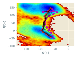
The trajectories of the image coordinates are written in the 6_rpath_prod/rp{}.rpath files. By observing these coordinates, we can easily track the evolution of the pathway. In the figure below, the purple line represents the initial pathway, black lines represent intermediate pathways during the sampling., and the red line is the final converged pathway (representing the minimum free energy path).
7. Umbrella sampling along the minimum free energy path
In the previous step, we obtained the converged pathway (minimum free energy pathway) connecting the alpha-helix and beta-sheet structures. In order to characterize the free energy profile along this pathway. we next use the umbrella sampling method to obtain the free energy surface. The umbrella sampling method has been widely used to calculate the free energy profile of the system along some collective variables. In this method, several restraint potentials are applied to the system along those collective variables, and histograms of the collective variables are obtained by using a reweighting algorithm. It should be noted that sufficient phase space overlaps are required for subsequent reweighting analysis, such as MBAR or WHAM.
# Change diretory
$ cd 7_umbrella/

# Run umbrella sampling
$ mpirun -np 16 /home/usr/GENESIS/bin/spdyn run.inp | tee run.log
The content of run.inp is shown below. Again, the reference values reference[12] for the restraints (image coordinates) are automatically replaced with those embedded in the restart files (in this case, those of the last snapshots in the replica path sampling). Please note that rpath_period and delta in [RPATH]should be set to 0 in umbrella sampling. Also, proper force constants are required for the sufficient phase space overlap between two adjacent replicas.
[INPUT]
topfile          = ../toppar/top_all36_prot.rtf
parfile          = ../toppar/par_all36_prot.prm
strfile          = ../toppar/toppar_water_ions.str
psffile          = ../1_setup/wbox.psf
pdbfile          = ../1_setup/start.pdb
rstfile          = ../6_rpath_prod/rp.{}.rst

[OUTPUT]
logfile          = umb.{}.log
dcdfile          = umb.{}.dcd
rstfile          = umb.{}.rst
rpathfile        = umb.{}.rpath

[ENERGY]
forcefield       = CHARMM
electrostatic    = PME
switchdist       = 10.0
cutoffdist       = 12.0
pairlistdist     = 13.5
vdw_force_switch = YES
pme_nspline      = 4
pme_max_spacing  = 1.2

[DYNAMICS]
integrator       = VVER
nsteps           = 200000
timestep         = 0.002
eneout_period    = 1000
crdout_period    = 1000
rstout_period    = 1000
nbupdate_period  = 10

[CONSTRAINTS]
rigid_bond       = YES

[ENSEMBLE]
ensemble         = NPT
tpcontrol        = BUSSI
temperature      = 300.0
pressure         = 1.0
isotropy         = ISO

[BOUNDARY]
type             = PBC

[RPATH]
nreplica         = 16
rpath_period     = 0
delta            = 0
rest_function    = 1 2

[SELECTION]
group1           = atomindex:15
group2           = atomindex:17
group3           = atomindex:19
group4           = atomindex:25
group5           = atomindex:27

[RESTRAINTS]
nfunctions       = 2

function1        = DIHED
constant1        = 20.0 20.0 20.0 20.0 20.0 20.0 20.0 20.0 \
                   20.0 20.0 20.0 20.0 20.0 20.0 20.0 20.0
reference1       = 0.0 0.0 0.0 0.0 0.0 0.0 0.0 0.0 \
                   0.0 0.0 0.0 0.0 0.0 0.0 0.0 0.0
select_index1    = 1 2 3 4 # PHI

function2        = DIHED
constant2        = 20.0 20.0 20.0 20.0 20.0 20.0 20.0 20.0 \
                   20.0 20.0 20.0 20.0 20.0 20.0 20.0 20.0
reference2       = 0.0 0.0 0.0 0.0 0.0 0.0 0.0 0.0 \
                   0.0 0.0 0.0 0.0 0.0 0.0 0.0 0.0
select_index2    = 2 3 4 5 # PSI
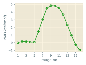
8. MBAR analysis of the free energy profile along the pathway
In this step, we analyze the output of the umbrella sampling simulation and evaluate the free energy profile along the converged pathway using the mbar_analysis tool in GENESIS. First, we use trj_analysis tool to obtain the collective variable (Φ and Ψ) file of each replica. Then, we use the “last_path.sh” shell script to produce a file (“last.path”) containing the image coordinates of the final converged minimum free energy pathway. In the last step, we use the mbar_analysis tool to analyze the collective variable files and output the free energy profile along the images, including the weight of each frame in every replica.
# Change directory
$ cd 8_mbar/

# Analyze the trajectories and obtain the collective variable files
$ ./trj_analysis.sh

# Obtain the path file of the final pathway
$ ./last_path.sh

# Obtain the free energy profile along the converged pathway with MBAR
$ /home/usr/GENESIS/bin/mbar_analysis mbar.inp | tee mbar.log
The content of mbar.inp is shown below. pathfile=last.path refers to the path file of the final converged pathway. cvfile=umb.{}.cv refers to the collective variable files.
[INPUT]
psffile            = ../1_setup/wbox.psf  # PSF file
pdbfile            = ../1_setup/start.pdb # PDB file
pathfile           = last.path            # path file
cvfile             = umb.{}.cv            # collective variable file

[OUTPUT]
fenefile           = output.fene          # free energy file
weightfile         = {}.weight            # weight file

[MBAR]
dimension          = 1       # dimension of the free energy profile
num_replicas       = 16      # number of replicas
input_type         = CV      # type of input file
nblocks            = 1
newton_iteration   = 100
temperature        = 300.0
target_temperature = 300.0
tolerance          = 10E-08
rest_function1     = 1 2
read_ref_path      = 0       # reference for each replica is defined explicitly

[RESTRAINTS]
constant1          = 0.001523 0.001523 0.001523 0.001523 \
                     0.001523 0.001523 0.001523 0.001523 \
                     0.001523 0.001523 0.001523 0.001523 \
                     0.001523 0.001523 0.001523 0.001523
reference1         = -61.478 -69.866 -77.478 -87.199 \
                     -93.803 -88.043 -88.675 -86.060 \
                     -85.670 -81.218 -80.901 -83.599 \
                     -77.368 -72.097 -66.649 -61.810
is_periodic1       = YES
box_size1          = 360.0

constant2          = 0.001523 0.001523 0.001523 0.001523 \
                     0.001523 0.001523 0.001523 0.001523 \
                     0.001523 0.001523 0.001523 0.001523 \
                     0.001523 0.001523 0.001523 0.001523
reference2         = -42.694 -31.873 -20.492 -10.852 \
                      1.0190  13.357  27.033  40.473 \
                      54.157  67.105  80.787  94.209 \
                      106.38  119.02  131.58  144.39
is_periodic2       = YES
box_size2          = 360.0
Written by Yasuhiro Matsunaga@RIKEN Computational biophysics research team
Created August 26, 2016
Updated By Weitong Ren@RIKEN Theoretical molecular science laboratory
Nov 15, 2019