12.1 gREST simulation of alanine-tripeptide in water
Contents
In this tutorial, we illustrate how to perform and analyze the replica exchange with solute tempering (REST) simulations for alanine tri-peptide. REST was originally designed by Berne et al.[1, 2] to improve the performance of temperature replica exchange MD (T-REMD) simulations. Instead of increase the temperature of the whole system, temperature of the “solute” region is virtually increased. This modification significantly reduces the required number of replicas. In GENESIS, new scheme of REST, referred to as generalized REST (gREST) [3], is implemented. In gREST, the solute region is defined as a part of a molecule and/or a part of the potential energy terms. The rational choice of the solute region in the gREST framework effectively limits the energy space covered in REST and reduces the number of required replica.
Preparation
First of all, let’s download the tutorial file (tutorial19-12.1.zip ). This tutorial consists of five steps: 1) system setup (12.1.1), 2) energy minimization and pre-equilibration (12.1.2), 3) equilibration (12.1.3), 4) production run (12.1.4), and 5) trajectory analysis (1.2.5). Control files for GENESIS are already included in the download file. Please refer to Tutorial 1.1 for general setup.
# Download the tutorial file
$ cd /home/user/GENESIS/Tutorials
$ mv ~/Downloads/tutorial19-12.1.zip ./
$ unzip tutorial19-12.1.zip
$ cd tutorial-12.1
$ ls
1_setup  2_minimize-pre-equil  3_equilibrate  4_production  5_analysis
$ ln -sf ../../Others/CHARMM/toppar .
Since we use the CHARMM force field, we make a symbolic link to the CHARMM toppar directory (see Tutorial 2).
1. Setup
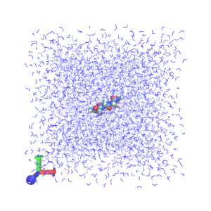
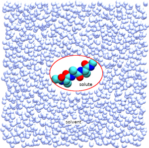
The input files to be used are already prepared in the 1_setup directory. In this directory, we have wbox.pdb (coordinate file) and wbox.psf (CHARMM structure file). The system is composed of one alanine tripeptide and 3,939 TIP3P waters. The initial box size is (x, y, z) = (50.2Å, 50.2Å, 50.2Å). The peptide forms a fully extended conformation with the backbone dihedral angle (φ, ψ) = (180°, 180°). This model was created using CHARMM and VMD (see “./1_setup/build/” if you are interested in the modeling). In addition to these files, par_all36m_prot.prm (CHARMM parameter file), top_all36_prot.rtf (CHARMM topology file), and toppar_water_ions.str(CHARMM topology and parameter file for TIP3P water and ions) in the toppar directory are required for the simulation.
# Change directory for the system setup
$ cd 1_setup
$ ls
build wbox.pdb wbox.psf

# View the initial structure
$ vmd wbox.pdb -psf wbox.psf
2. Minimization and pre-equilibration
Non-physical steric clashes or non-equilibrium geometries in the initial structure must be resolved before the REMD simulation. Here, we do this via four steps: 1) minimization (step2.1), 2) equilibration in NVT ensemble (step2.2), 3) relaxation of the simulation box in NPT ensemble with positional restraints (step2.3), and 4) equilibration in NPT ensemble without positional restraints. In the 2_minimize_pre-equil directory, all control files “step2.*.inp” are given.
# Change directory
$ cd 2_minimize_pre-equi
$ ls
step2.1.inp step2.2.inp step2.3.inp step2.4.inp
2.1. Minimization
We first minimize the potential energy of the system. atdyn and spdyn support the steepest descent algorithm for minimization, which moves atoms proportionally to their negative gradients of the potential energy. Here we use spdyn, but you can also use atdyn:
The control file “step2.1.inp” is as follows:
[INPUT]
topfile = ../toppar/top_all36_prot.rtf     # topology file
parfile = ../toppar/par_all36m_prot.prm     # parameter file
strfile = ../toppar/toppar_water_ions.str  # stream file
psffile = ../1_setup/wbox.psf              # protein structure file
pdbfile = ../1_setup/wbox.pdb              # PDB file
reffile = ../1_setup/wbox.pdb              # PDB file for restraints

[OUTPUT]
dcdfile    = step2.1.dcd   # DCD trajectory file
rstfile    = step2.1.rst   # restart file

[ENERGY]
forcefield       = CHARMM   # CHARMM force field
electrostatic    = PME      # Particle Mesh Ewald method
switchdist       = 10.0     # switch distance
cutoffdist       = 12.0     # cutoff distance
pairlistdist     = 13.5     # pair-list distance
vdw_force_switch = YES      # force switch option for van der Waals
pme_nspline      = 4        # order of B-spline in [PME]
pme_max_spacing  = 1.0      # max grid spacing
contact_check    = YES      # avoid calculation failure due to atomic crash

[MINIMIZE]
method           = SD       # Steepest descent method
nsteps           = 2000     # number of minimization steps
eneout_period    =  100     # energy output period
crdout_period    =  100     # coordinates output period
rstout_period    = 2000     # restart output period
nbupdate_period  =   10     # nonbond update period

[BOUNDARY]
type             = PBC      # periodic boundary condition
box_size_x       = 50.200   # box size (x) in [PBC]
box_size_y       = 50.200   # box size (y) in [PBC]
box_size_z       = 50.200   # box size (z) in [PBC]

[SELECTION]
group1           = sid:PROA and heavy

[RESTRAINTS]
nfunctions       = 1        # number of functions
function1        = POSI     # restraint function type
direction1       = ALL      # direction
constant1        = 1.0      # force constant
select_index1    = 1        # restrained groups
If you use AMBER force field parameter set, you specify file names of
prmtopfile (amber prmtop format file) and ambcrdfile (rst7 ascii format file) instead of topfile, prmfile, strfile, crdfile and psffile in [INPUT] section (see this page).
In [ENERGY] section, contact_check option is used to avoid the failure due to bad steric clash often included in your initial structures. This option is available in minimization step only.
In [BOUNDARY] section, the boundary conditions and the simulation box size are set. box_size_x, box_size_y, box_size_z specify the box dimensions of the system, and must be given in the first minimization step.
In [RESTRAINTS] section, positional restraints are applied to the atom group “group1” which consists of heavy atoms of the peptide. This atom group is defined in the [SELECTION] section. The restraints are imposed with respect to the reference coordinates given by reffile in [INPUT] section.
2.2. Equilibration of the system at 300 K
Next, we equilibrate the system at 300 K in NVT ensemble for 10 ps. In the following MD simulations, we use multiple time step integrator, r-RESPA (VRES, timestep of 2.5 fs) with BUSSI’s thermostat (see Recommended control parameters for ver. 1.4). The following is the important options in the control file (step2.2.inp).
[DYNAMICS]
integrator       = VRES      # [LEAP,VVER,VRES]
nsteps           = 5000      # number of MD steps
timestep         = 0.0025    # timestep (ps)
nbupdate_period  = 10        # pairlist update period
elec_long_period = 2         # period of reciprocal space calculation
thermostat_period = 10       # period of thermostat update
barostat_period  = 10        # period of barostat update
eneout_period    = 10        # energy output period
crdout_period    = 100       # coordinates output period
rstout_period    = 5000      # restart output period

[CONSTRAINTS]
rigid_bond       = YES       # use SHAKE/RATTLE
fast_water       = YES       # use SETTLE

[ENSEMBLE]
ensemble         = NVT       # [NVE,NVT,NPT]
tpcontrol        = BUSSI     # thermostat and barostat
temperature      = 300.00    # K

[BOUNDARY]
type             = PBC       # periodic boundary condition

[SELECTION]
group1           = sid:PROA and heavy

[RESTRAINTS]
nfunctions       = 1        # number of functions
function1        = POSI     # restraint function type
direction1       = ALL      # direction
constant1        = 1.0      # force constant
select_index1    = 1        # restrained groups
[CONSTRAINTS] section specifies constraints during a simulation. “rigid_bond” is a keyword to use SHAKE algorithm for the peptide molecule. For water molecules, a faster algorithm (SETTLE algorithm) is automatically applied if rigid_bond = YES. In [BOUNDARY] section, we do not specify the box dimensions, because the values are read from the rstfile.
2.3. Relaxation of the simulation box
After the system reached the desired temperature 300.00 K, we relax the simulation box in NPT ensemble at 300 K and 1 atm for 10 ps. The following is the important options in the control file (step2.3.inp).
[ENSEMBLE]
ensemble         = NPT       # [NVE,NVT,NPT]
tpcontrol        = BUSSI     # thermostat and barostat
pressure         = 1.0       # atm
temperature      = 300.00    # K

[SELECTION]
group1           = sid:PROA and heavy

[RESTRAINTS]
nfunctions       = 1        # number of functions
function1        = POSI     # restraint function type
direction1       = ALL      # direction
constant1        = 1.0      # force constant
select_index1    = 1        # restrained groups
2.4. Equilibration with no positional restraints
Finally we run an additional 10-ps pre-equilibration simulation in NPT ensemble (step2.4.inp). In this step, we relax all atom positions including the peptide atoms without positional restraints (removes [RESTRAINTS]section).
Please run above calculations as follows to minimize and pre-equilibrate the system.
# Energy minimization
# OMP_NUM_THREADS is a number of threads per a MPI process
$ export OMP_NUM_THREADS=3
$ mpirun -np 8 /home/user/GENESIS/bin/spdyn step2.1.inp > step2.1.log

# Equilibration in the NVT ensemble with restratins (VRES, timestep of 2.5 fs)
$ mpirun -np 8 /home/user/GENESIS/bin/spdyn step2.2.inp > step2.2.log

# Equilibration in the NPT ensemble with restratins (VRES, timestep of 2.5 fs)
$ mpirun -np 8 /home/user/GENESIS/bin/spdyn step2.3.inp > step2.3.log

# Equilibration in the NPT ensemble (VRES, timestep of 2.5 fs)
$ mpirun -np 8 /home/user/GENESIS/bin/spdyn step2.4.inp > step2.4.log
3. Equilibration
In this step, we equilibrate the system for each replica without replica exchange. The control file of REST is very similar to that of T-REMD. The only difference is that REST needs select_indexN to specify the “solute” region. The rest of system is regarded as “solvent”. In this example, we define the the alanine tri-peptide molecule as the solute region (group1 = ai:1-42 in [SELECTION] section). Four replicas are used over the solute temperature range of 300.00 K – 351.26 K (parameters1 = 300.00 318.12 337.14 351.26 in [REMD] section). In default, all of potential energy terms are treated as the solute (param_type1 = ALL in [REMD] section). If you want to treat a part of potential energy terms as the solute, param_typeN parameter may be modified (e.g. param_type1 = D CM to specify only dihedral and CMAP terms as solute.). In the 3_equilibration directory, the control file “step3.inp” is given.
# Change directory
$ cd 3_equilibration
$ ls
step3.inp

# Execute equilibration run
$ export OMP_NUM_THREADS=3
$ mpirun -np 8 /home/user/GENESIS/bin/spdyn step3.inp > step3.log
The following is the important options of the control file (step3.inp).
[OUTPUT]
dcdfile  = step3_rep{}.dcd       # DCD trajectory file
rstfile  = step3_rep{}.rst       # restart file
remfile  = step3_rep{}.rem       # replica exchange ID file
logfile  = step3_rep{}.log       # log file of each replica

[REMD]
dimension        = 1           # number of parameter types
exchange_period  = 0           # NO exchange for equilibration
iseed            = 3141592

type1           = REST          # Replica Exchange with Solute Tempering
nreplica1       = 4             # number of replicas
parameters1     = 300.00 318.12 337.14 351.26 # list of solute temperatures
select_index1   = 1             # solute region selection
param_type1     = ALL          # function types
                                # valid keywords are:
                                # ALL (default), BOND, ANGLE,
                                # DIHEDRAL, IMPROPER, CMAP,
                                # CHARGE LJ...
                                # See manual for further details.

[SELECTION]
group1        = ai:1-42
4. Production
Now, we are ready to perform REST simulation. One needs to modify the control file for the equilibration such that the exchange_period has a non-zero value (e.g. 1000 steps (2.5 ps)) and [INPUT] and [OUTPUT] files are properly refered. In order to analyze the free energy, you need to select the grest_analysis=YES in [REMD]. The option enables calculation of energies with different solute temperatures. The energies with different solute temperatures of each replica are written in step4_1_rep{}.ene.
To run the simulation, goto 4_production/ directory and execute the production run.
# change directory
$ cd 4_production
$ ls
step4.1.inp step4.2.inp step4.3.inp

# Execute equilibration run
$ export OMP_NUM_THREADS=3
$ mpirun -np 8 /home/user/GENESIS/bin/spdyn step4.1.inp > step4.1.log
The important part of the control file (step4.1.inp) is as follows:
[INPUT]
rstfile = ../3_equilibration/step3_rep{}.rst  # restart file

[OUTPUT]
dcdfile  = step4_1_rep{}.dcd       # DCD trajectory file
rstfile  = step4_1_rep{}.rst       # restart file
remfile  = step4_1_rep{}.rem       # replica exchange ID file
logfile  = step4_1_rep{}.log       # log file of each replica
enefile  = step4_1_rep{}.ene       # energy file of each replica

[REMD]
dimension        = 1           # number of parameter types
exchange_period  = 1000        # NO exchange for equilibration
iseed            = 3141592

type1            = REST
nreplica1        = 4           # number of replicas
parameters1      = 300.00 318.12 337.14 351.26 # list of solute temperatures
select_index1    = 1
analysis_grest   = YES

[SELECTION]
group1           = ai:1-42
5. Analysis
This section describes how to analyze REST trajectories. We first check the performance of replica exchange (calculate the acceptance ratio (5-1_calc_ratio) and check random walks (5-2_plot_index)), next we sort the dcd files for further analysis (5-3_sort_dcd), and finally draw the potential of mean force using MBAR (5-4_mbar). The control files for the analyses are given in the 5_analysis directory.
# Change directory
$ cd ../5_analysis
$ ls
5-1_calc_ratio  5-2_plot_index  5-3_sort_dcd 5-4_mbar
5.1. Calculate the acceptance ratio
We first check the acceptance ratio of replica exchange which represents the efficiency of REMD simulations. The acceptance ratio is displayed in the “step4.1.log“, and we examine the value from the last exchange step. The script “calc_ratio.sh” can be used for the analysis.
# Change directory
$ cd 5-1_calc_ratio

# Make the file executable and use it
$ chmod u+x calc_ratio.sh
$ ./calc_ratio.sh

1 > 2 0.55
2 > 3 0.65
3 > 4 0.75
The script “calc_ratio.sh” contains the following commands:
# Get acceptance ratios between adjacent parameter IDs
grep "  1 >     2" ../../4_production/step4.1.log | tail -1  > acceptance_ratio.dat
grep "  2 >     3" ../../4_production/step4.1.log | tail -1 >> acceptance_ratio.dat
grep "  3 >     4" ../../4_production/step4.1.log | tail -1 >> acceptance_ratio.dat

# Calculate the ratios
awk '{print $2,$3,$4,$6/$8}' acceptance_ratio.dat
5.2. Plot time courses of replica indices and temperatures
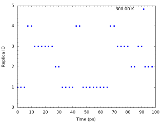
Next, we examine the random walks of replica indices at different solute temperatures. We take the values of the “ParmIDtoRepID” lines for the solute temperature of interest, for example 300 K (first column), from step4.1.log . The script “plot_index.sh” can be used for the analysis.
# Change directory
$ cd ../5-2_plot_index

# Make the file executable and use it
$ chmod u+x plot_index.sh
$ ./plot_index.sh
$ chmod u+x plot_temperature.sh
$ ./plot_temperature.sh
The script “plot_index.sh” contains the following commands:
# Get replica IDs in each snapshot
grep "ParmIDtoRepID:" ../../4_production/step4.1.log | sed 's/ParmIDtoRepID:/ /' > param.dat

# Plot replica IDs in each snapshot
cat << EOF > tmp.plt
set term png
set yrange [0:5]
set mxtics
set mytics
set xlabel "Time (ps)"
set ylabel "Replica ID"
set output "output_index1.png"
plot "param.dat" using (\$0*2.5):1 with points pt 5 ps 0.5 lc rgb "blue" title "300.00 K"
set output "output_index2.png"
plot "param.dat" using (\$0*2.5):2 with points pt 5 ps 0.5 lc rgb "cyan" title "318.12 K"
set output "output_index3.png"
plot "param.dat" using (\$0*2.5):3 with points pt 5 ps 0.5 lc rgb "green" title "337.14 K"
set output "output_index4.png"
plot "param.dat" using (\$0*2.5):4 with points pt 5 ps 0.5 lc rgb "red" title "351.26 K"
EOF

gnuplot tmp.plt
rm -rf tmp*
The following is the random walk of replica indices at the solute temperature of 300.00 K as an example.
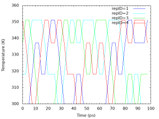
Similarly, we examine the random walks of solute temperatures for 4 replica indices. We take the values of the “Parameter :” lines for each replica from step4.1.log. The script “plot_temperature.sh” can be used for the analysis.
# Get replica temperatures in each snapshot
grep "Parameter    :" ../../4_production/step4.1.log | sed 's/Parameter    :/ /' > temperature.dat

# Plot replica temperatures in each snapshot
cat << EOF > tmp.plt
set term png
set mxtics
set mytics
set xlabel "Time (ps)"
set ylabel "Temperature (K)"
set output "output_temperature.png"
plot "temperature.dat" using (\$0*2.5):1  with lines lc rgb "blue" title "repID=1 ", "temperature.dat" using (\$0*2.5):2  with lines lc rgb "cyan" title "repID=2 ", "temperature.dat" using (\$0*2.5):3  with lines lc rgb "green" title "repID=3 ", "temperature.dat" using (\$0*2.5):4  with lines lc rgb "red" title "repID=4 "
EOF

gnuplot tmp.plt
rm -rf tmp*
The following is the random walks of solute temperatures for each replica.
5.3. Convert trajectories
Raw output trajectories contain snapshots from various solute temperature. To get ensemble of specific solute temperature, one may use remd_convert utility which sorts the trajectories based on the information written in the remfiles. The procedure is basically identical to that for T-REMD trajectories.
# Change directory
$ cd ../5-3_sort_dcd

# Execute the job
$ /home/usr/GENESIS/bin/remd_convert remd_conv.1.inp > remd_conv.1.log
This example sorts the trajectory of the solute temperature of 300.00 K (parameterID = 1) (convert_type = PARAMETER, convert_ids = 1 in [OPTION] section). The system is aligned to the backbone of central alanine during the sorting (fitting_atom = 2 in [FITTING] section, group2 = resno:2 and (an:N or an:CA or an:C or an:O in [SELECTION] section), and the water molecules are removed from the sorted trajectory (trjout_atom = 1 in [OPTION] section, group1 = ai:1-42 in [SELECTION] section).
The control file “remd_conv.1.inp” is as follows:
[INPUT]
psffile = ../../1_setup/wbox.psf
reffile = ../../1_setup/wbox.pdb
dcdfile = ../../4_production/step4_1_rep{}.dcd # see remd_conv.sh
remfile = ../../4_production/step4_1_rep{}.rem # see remd_conv.sh

[OUTPUT]
trjfile = remd_1_param{}.dcd

[SELECTION]
group1          = ai:1-42   # only tri-alanine
group2          = resno:2 and (an:N or an:CA or an:C or an:O) # backbone of 2nd ALA

[FITTING]
fitting_method  = TR+ROT    # center-of-mass translation + rotation fitting
fitting_atom    = 2         # fitting to backbone of central alanine
mass_weight     = YES       # mass-weighted fitting

[OPTION]
check_only      = NO
convert_type    = PARAMETER
convert_ids     =
num_replicas    = 4
nsteps          = 40000
exchange_period = 1000
crdout_period   = 100       # trjectory output frequency in REMD
eneout_period   = 10        # trjectory output frequency in REMD
trjout_format   = DCD
trjout_type     = COOR+BOX
trjout_atom     = 1         # output only tri-alanine moiety
pbc_correct     = NO        # nothing will happen when water mols excluded
If convert_ids = , all trajectories are written. One can sort the trajectory for the highest temperature (351.26 K, parameterID = 4) by specifying convert_ids = 4 in [OPTION] section, for example.
“num_replicas“, “nsteps“, “exchange_period“, and “eneout_period” are set to the save values as those in the REST control file.
One can check the sorted trajectory by following commands:
# Check the sorted dcd file for ParameterID 1 (300.00 K)
$ vmd ../../1_setup/build/ala3.psf -dcd ./remd_1_param1.dcd
5.4. Free energy analysis using MBAR
Finally, we calculate the free energy profile of the alanine tripeptide along the end-to-end distance using MBAR. There are 4 steps to do this: 1) calculate the end-to-end distance using trj_analysis, 2) sort the energies at different solute temperatures based on the information written in the remfiles using remd_convert, 3) perform MBAR analysis using mbar_analysis, 4) calculate the potential of mean force (PMF) using pmf_analysis. The control files for each step are given in the 5_analysis directory.
# Change directory
$ cd ../5-4_mbar
$ ls
5-4-1_distance 5-4-2_remd_convert 5-4-3_mbar 5-4-4_pmf
1) calculate the end-to-end distance using trj_analysis.
For MBAR analysis, we calculate the end-to-end distances for all sorted trajectories at different solute temperatures (inp1, inp2, inp3, and inp4).
# Change directory
$ cd 5-4-1_distance
$ ls
inp1 inp2 inp3 inp4

# Execute the job
$ /home/usr/GENESIS/bin/trj_analysis inp1 > log1
$ /home/usr/GENESIS/bin/trj_analysis inp2 > log2
$ /home/usr/GENESIS/bin/trj_analysis inp3 > log3
$ /home/usr/GENESIS/bin/trj_analysis inp4 > log4
The control file “inp1” is as follows:
[INPUT]
psffile        = ../../../1_setup/build/ala3.psf
reffile        = ../../../1_setup/build/ala3.pdb

[OUTPUT]
disfile        = param1.dis

[TRAJECTORY]
trjfile1       = ../../5-3_sort_dcd/remd_1_param1.dcd
md_step1       = 40000           # number of MD steps
mdout_period1  = 100             # MD output period
ana_period1    = 100             # analysis period
repeat1        = 1
trj_format     = DCD             # (PDB/DCD)
trj_type       = COOR+BOX        # (COOR/COOR+BOX)
trj_natom      = 0               # (0:uses reference PDB atom count)

[OPTION]
check_only     = NO              # (YES/NO)
distance1      = PROA:1:ALA:OY PROA:3:ALA:HNT
The sorted trajectory for parameter ID = 1 (solute temperature of 300.00 K) is specified (
trjfile1 = ../../5-3_sort_dcd/remd_1_param1.dcd in [TRAJECTORY] section).
The sorted trajectory has the coordinates of alanine tripeptide only, the corresponding psfile and reffile are specified (psffile = ../../../1_setup/build/ala3.psf and reffile = ../../../1_setup/build/ala3.pdb in [INPUT] section).
This produces 4 “*.dis” files containing the end-to-end distances for 4 sorted trajectories. For example, param1.dis is as follows:
$ less param1.dis

1     10.248
2      9.606
3      9.610
4      9.721
5      9.828
6      9.979
2) sort the energies using remd_convert.
# Change directory
$ cd ../5-4-2_remd_convert
$ ls remd_conver.inp
# Execute the job
$ /home/usr/GENESIS/bin/remd_convert remd_convert.inp > remd_convert.log
The control file “remd_convert.inp” is as follows:
[INPUT]

remfile        =  ../../../4_production/step4_1_rep{}.rem   # remfile of gREST
enefile        =  ../../../4_production/step4_1_rep{}.ene   # enefile of gREST

[OUTPUT]

enefile        = eneout_param{}  # sorted enefile

[OPTION]

check_only      = NO
convert_type    = PARAMETER
convert_ids     =
num_replicas    = 4
nsteps          = 40000            # number of steps of gREST
exchange_period = 1000               # exchange frequency of gREST
crdout_period   = 100                # output frequency of enefile of gREST
The program also sorts the energies of all solute temperatures (convert_type = PARAMETER and blank in convert_ids in [OPTION] section).
This produces 4 “eneout_param*” files containing the energies at different solute temperatures at the snapshots of each replica. For example, eneout_param1 is as follows:
100 -38574.8109 -38574.4224 -38573.9782 -38573.6316
200 -38566.8707 -38566.6783 -38566.4211 -38566.2027
300 -38480.4939 -38480.5933 -38480.6074 -38480.5707
400 -38475.4540 -38475.2750 -38475.0249 -38474.8082
500 -38598.4846 -38598.2298 -38597.9120 -38597.6515
600 -38440.0780 -38439.5551 -38438.9825 -38438.5481
3) perform MBAR analysis using mbar_analysis.
# Change directory
$ cd ../5-4-3_mbar
$ ls
mbar.inp

# Execute the job
$ /home/usr/GENESIS/bin/mbar_analysis mbar.inp > mbar.log
The control file ” mbar.inp” is as follows:
[INPUT]
cvfile             = ../energy/eneout_param{} # input cv file

[OUTPUT]
fenefile           = fene.dat
weightfile         = weight{}.dat

[MBAR]
nreplica           = 4
input_type         = REST
dimension          = 1
nblocks            = 1
temperature        = 300.00
target_temperature = 300.00
This produces “fene.dat” file containing the evaluated relative free energies and 4 “weight*.dat” files containing the weights of each snapshot for each replica. For example, weight1.dat is as follows:
$ less weight1.dat
100 7.326314464464978E-004
200 5.985010541708708E-004
300 3.836388573225608E-004
400 5.903579307509812E-004
500 6.434845172380442E-004
600 8.118218870078299E-004
4) calculate the potential of mean force (PMF) using pmf_analysis.
# Change directory
$ cd ../5-4-4_pmf

$ ls
pmf.inp

# Execute the job
$ /home/usr/GENESIS/bin/pmf_analysis pmf.inp > pmf.log
The control file “pmf.inp” is as follows:
[INPUT]
cvfile       = ../distance/param{}.dis
weightfile   = ../mbar/weight{}.dat

[OUTPUT]
pmffile      = dist.pmf

[OPTION]
nreplica     = 4             # number of replicas
dimension    = 1             # dimension of cv space
temperature  = 300.0
grids1       = 0 15 101      # (min max num_of_bins)
band_width1  = 0.1
is_periodic1 = NO            # periodicity of cv1
This produces “*.pmf” file as follows:
7.500000000000000E-002 Infinity Infinity
0.225000000000000 Infinity Infinity
0.375000000000000 Infinity Infinity
0.525000000000000 Infinity Infinity
(skip)
9.82500000000000 0.129245385819335 0.108514857241108
9.97500000000000 0.000000000000000E+000 0.000000000000000E+000
10.1250000000000 0.104056748685860 3.870802986704869E-002
10.2750000000000 0.109733337874484 6.153261485211675E-002
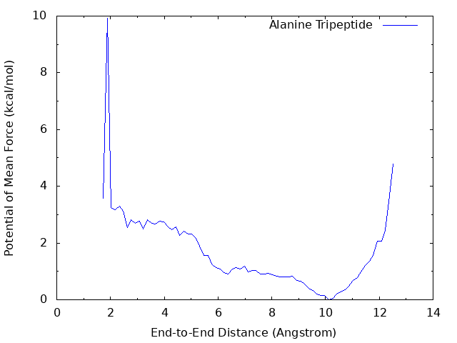
By plotting the “dist.pmf“, one obtain the following graph.

The PMF from a well converged simulation shows that there is a global energy minimum around r = 10 Å, and a local energy minimum around r = 2 Å which corresponds to the α-helix conformation with the hydrogen bond between OY and HNT. The above graph misses the local minimum becase of insufficient sampling (100 ps / replica). The following graph is obtained from the longer sampling (10 ns / replica).
5.5. Hints
- The output trajectory is an ordinary dcd file, you can use various analysis programs for these files.
- REST can be combined with REUS (H-REMD); huge computational resources required, though.
- Multidimensional REST might be possible; not of great use, though.
References
- P. Liu, B. Kim, R. A. Friesner, B. J. Berne, Replica exchange with solute tempering: A method for sampling biological systems in explicit water. Proc. Natl. Acad. Sci. U.S.A.102, 13749–13754 (2005).
- L. Wang, R. A. Friesner, B. J. Berne, Replica exchange with solute scaling: A more 683efficient version of replica exchange with solute tempering (REST2). J. Phys. Chem. B 115, 9431–9438 (2011).
- M. Kamiya, Y. Sugita, Flexible selection of the solute region in replica exchange with solute tempering: Application to protein-folding simulations. J. Chem. Phys. 149, 072304 (2018)
- A. Patriksson & D. van der Spoel, “A temperature predictor for parallel tempering simulations.” Phys. Chem. Chem. Phys., 10, 2073-2077 (2008).
Written by Motoshi Kamiya@RIKEN Computational biophysics research team
Mar 1, 2018
Updated Feb 25, 2019 by Yasuhiro Matsunaga
Updated Aug 31, 2019 by Suyong Re
Updated April 4, 2022 by Chigusa Kobayashi
Updated May 11, 2022 by Chigusa Kobayashi