1.2 All-atom MD simulation of POPC lipid bilayers
Files for this tutorial (charmm-gui.gtz)
Optional input file to wrap atoms into unit cell (tutorial1.2-crd_convert.inp)
Contents
Cell membranes have many biological roles such as substrate transport, signal transduction, and cell adhesion. By using GENESIS, the user can simulate biological membranes at the atomistic level. One of the difficulties in such simulations is initial setup of the bilayer structure or equilibration of the system. Because each lipid molecule has a random structure, it may take much time to equilibrate the whole system, if the initial structure has an ordered conformation. CHARMM-GUI is one of the useful tools to generate initial structures of lipid bilayers for MD simulations (S. Jo et al., 2007 ). It provides the automatic membrane builder for not only pure lipid bilayers but also protein-membrane systems. Recently, GENESIS format has been introduced into the CHARMM-GUI membrane builder as well as NAMD, GROMACS, AMBER, OpenMM, and CHARMM/OpenMM formats (J. Lee et al., 2015 ). Here, we explain how to simulate POPC (1-palmitoyl-2-oleoyl-sn-glycero-3-phosphocholine) lipid bilayers with GENESIS and CHARMM-GUI using the CHARMM C36 force fields (J. Klauda et al., 2010 ). Other sample control files for membrane simulations are also available here.
1.2.1 Setup initial structure with CHARMM-GUI
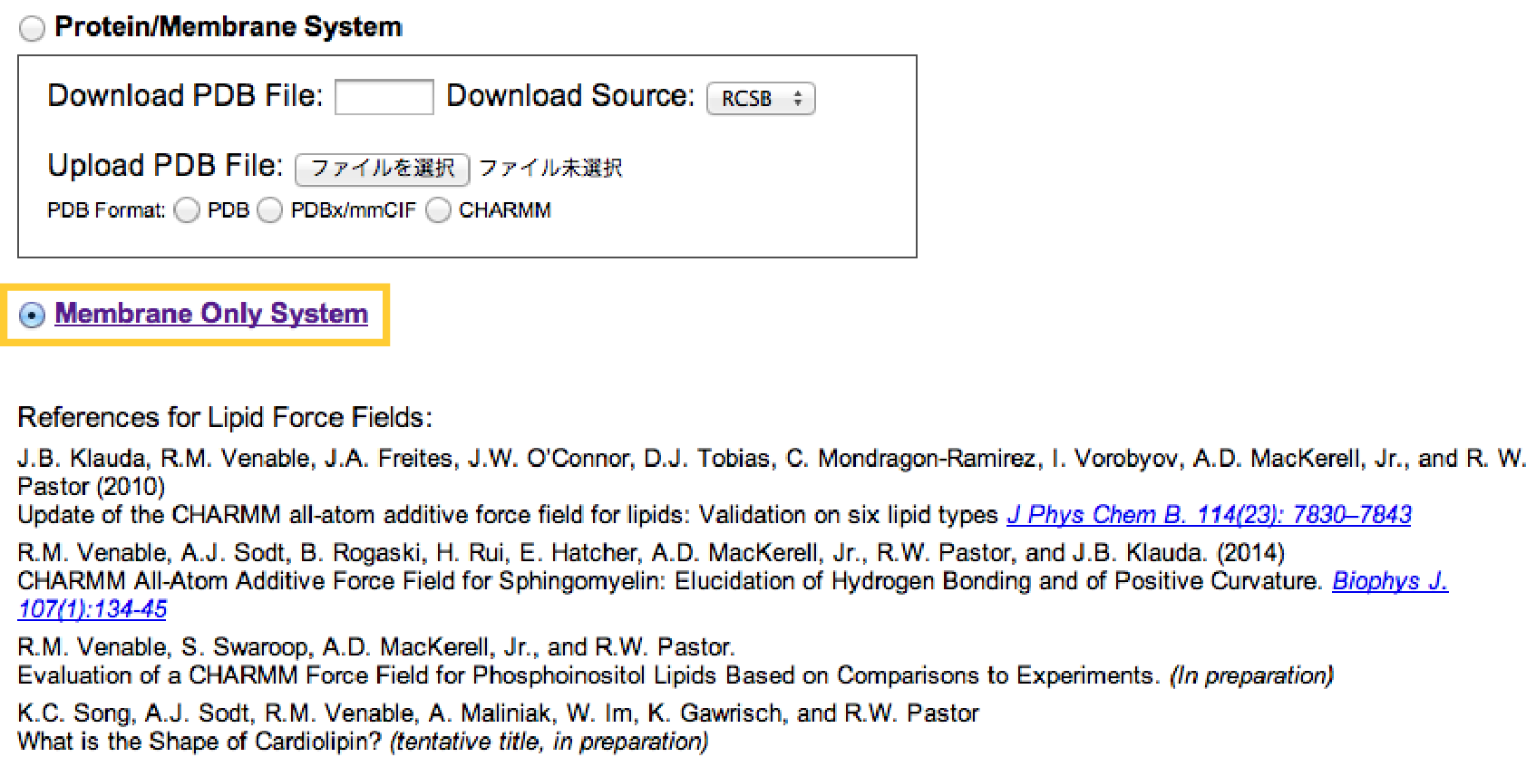
We use the Bilayer builder in the CHARMM-GUI. If the server is not working, files prepared by us included in the tutorial files (available from the link just below the title of this page) can be used instead. In this case, this section can be skipped. Now, let us build a POPC lipid bilayer. At the first step of the bilayer builder, we choose “Membrane Only System”:
In the next step, we decide the number of lipids and water molecules to be added in the system. Here, we put 40 POPC and 40 POPC lipids in the upper and lower leaflets, respectively (Note that these numbers might be a lower limit for stable MD simulation with spdyn). Because each lipid molecule has a certain area per lipid (Aexp = 68.3Å2 for POPC), the initial box size (X, Y) = (52.27Å, 52.27Å) can be estimated from sqrt{(number of lipids in one leaflet)*(area per lipid)}. 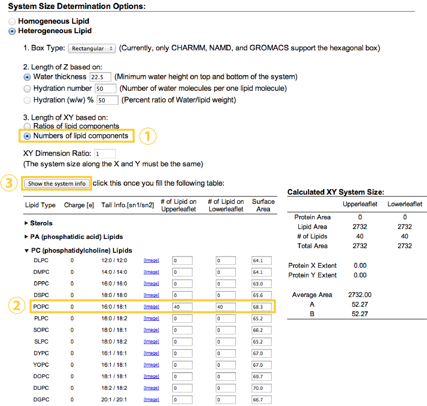
In the next steps, we add 0.15 M KCl in the system, mimicking the cellular environment, with the Monte Carlo method for ion placing. Then, we click “Next Step” three times. We check “GENESIS” in “Input Generation Options” and select the NPT ensemble at T = 303.15K in “Equilibration Options”. At this temperature, POPC bilayers show liquid phase rather than gel phase (Tm = 271K). After clicking the “Next Step”, we can download a set of input files for minimization, equilibration, and production runs for GENESIS at the final step of the membrane builder.

1.2.2 Simulation with GENESIS
First of all, let us see the PDB structure in the downloaded file by using VMD:
# make a new directory to do this tutorial and copy the downloaded file
$ mkdir tutorial-1.2
$ cd tutorial-1.2
$ cp ~/Download/charmm-gui.tgz ./

# check the downloaded files
$ tar -xzf charmm-gui.tgz
$ cd charmm-gui
$ vmd step5_assembly.pdb
We use this PDB file as the initial coordinates of the simulation. In the current working directory, there is the genesis directory, where several control files for GENESIS are contained:
$ cd genesis
$ ls
restraints                 step6.2_equilibration.inp  step6.6_equilibration.inp
step5_charmm2genesis.str   step6.3_equilibration.inp  step7_production.inp
step6.0_minimization.inp   step6.4_equilibration.inp
step6.1_equilibration.inp  step6.5_equilibration.inp
These control files are mainly composed of three steps: energy minimization (step6.0), equilibration (step6.1-6.6), and production runs (step7). In total, 8 simulations are carried out step by step. Basically, we do not need to edit these control files (If the user uses GENESIS1.0, pme_ngrid_x, y, and z should be set in the [ENERGY] section). During Step6.0-6.6, dihedral angle restraints are applied on some parts of the system to avoid unexpected structural change in the lipid molecule such as isomerization or cis-trans transition of double bonds. In the restraints directory, such restraint functions are defined, and they are called from the control files. Positional restraints are also imposed on z-coordinates of lipid phosphorous atoms in order to prevent undulation of the membrane plane. These restraint forces are gradually reduced to zero during the equilibration.
Let us check parameters in the control files (step6.0-step7) before running the simulation. For step7, we can see:
$ less step7_production.inp
:
[ENERGY]
forcefield        = CHARMM    # [CHARMM]
electrostatic     = PME       # [CUTOFF,PME]
switchdist        = 10.0      # switch distance
cutoffdist        = 12.0      # cutoff distance
pairlistdist      = 13.5      # pair-list distance
pme_nspline       = 4
water_model       = NONE
vdw_force_switch  = YES

[DYNAMICS]
integrator        = VVER      # [LEAP,VVER]
timestep          = 0.002     # timestep (ps)
nsteps            = 500000    # number of MD steps
crdout_period     = 1000
eneout_period     = 1000      # energy output period
rstout_period     = 1000
nbupdate_period   = 10

[CONSTRAINTS]
rigid_bond        = YES       # constraints all bonds involving hydrogen
fast_water        = YES
shake_tolerance   = 1.0D-10

[ENSEMBLE]
ensemble          = NPT       # [NVE,NVT,NPT]
tpcontrol         = LANGEVIN  # thermostat and barostat
temperature       = 303.15
pressure          = 1.0       # atm
gamma_t           = 1.0
gamma_p           = 0.05
isotropy          = SEMI-ISO

[BOUNDARY]
type              = PBC       # [PBC]
All control files already include optimal or well-established MD parameters. For example, in the [ENERGY] section, we specify switchdist = 10 Å, cutoffdist = 12 Å, and vdw_force_switch = YES, which are recommended in the membrane simulations with the CHARMM C36 force fields (J. Lee et al., 2015 ). We use the SHAKE/SETTLE algorithms for rigid bonds, and Langevin thermostat and barostat for temperature and pressure control. As for the pressure control, semi-isotropic pressure coupling is used. The equations of motion are integrated by the velocity Verlet method.
Let us carry out energy minimization, equilibration, and production runs with spdyn. Here, we use 16 MPI processors as an example. You can use a smaller or larger number of MPI processors as well. Since the system size is relatively large, it may take more than 10 minutes in some equilibration runs and more than 3 hours in the production run.
# 1000 step energy minimization
# with dihedral angle restraint (k = 250 kcal/mol)
#      z-positional restraint on P atoms (k = 2.5 kcal/mol/Å2)
$ export OMP_NUM_THREADS=1
$ mpirun -np 16 /home/user/genesis/bin/spdyn step6.0_minimization.inp > log6.0

# 25ps MD in the NVT ensemble
# with dihedral angle restraint (k = 250 kcal/mol)
#      z-positional restraint on P atoms (k = 2.5 kcal/mol/Å2)
$ mpirun -np 16 /home/user/genesis/bin/spdyn step6.1_equilibration.inp > log6.1

# 25ps MD in the NVT ensemble
# with dihedral angle restraint (k = 100 kcal/mol)
#      z-positional restraint on P atoms (k = 2.5 kcal/mol/Å2)
$ mpirun -np 16 /home/user/genesis/bin/spdyn step6.2_equilibration.inp > log6.2

# 25ps MD in the NVT ensemble
# with dihedral angle restraint (k = 50 kcal/mol)
#      z-positional restraint on P atoms (k = 1.0 kcal/mol/Å2)
$ mpirun -np 16 /home/user/genesis/bin/spdyn step6.3_equilibration.inp > log6.3

# 100ps MD in the NPT ensemble
# with dihedral angle restraint (k = 50 kcal/mol)
#      z-positional restraint on P atoms (k = 0.5 kcal/mol/Å2)
$ mpirun -np 16 /home/user/genesis/bin/spdyn step6.4_equilibration.inp > log6.4

# 100ps MD in the NPT ensemble
# with dihedral angle restraint (k = 25 kcal/mol)
#      z-positional restraint on P atoms (k = 0.1 kcal/mol/Å2)
$ mpirun -np 16 /home/user/genesis/bin/spdyn step6.5_equilibration.inp > log6.5

# 100ps MD in the NPT ensemble without any restraints
$ mpirun -np 16 /home/user/genesis/bin/spdyn step6.6_equilibration.inp > log6.6

# 1000ps MD in the NPT ensemble
$ mpirun -np 16 /home/user/genesis/bin/spdyn step7_production.inp > log7
At the last step, we obtain the coordinates trajectory file step7_procution.dcd.
1.2.3 Visualization of the trajectory
Let us visualize the trajectory file by using VMD:
$ vmd ../step5_assembly.pdb -psf ../step5_assembly.psf -dcd step7_production.dcd
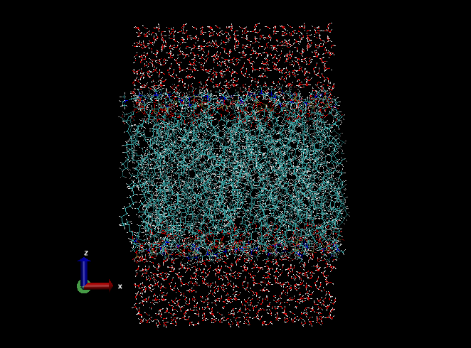
In the simulation, we can see that hydrophobic lipid tail groups fluctuate significantly and form random conformation. Water molecules are interacting with hydrophilic lipid head groups through hydrogen bonds. One of the important features of the lipid bilayers is that they are almost impermeable to ions because of the low dielectric environment in the hydrophobic core region.
In the VMD viewer window, we may find H-H bond in the TIP3P water, but it does not matter because it comes from definition of H-H bond in the PSF file for the SHAKE/SETTLE algorithms. We can also see that water molecules are spread out from the simulation box, but they are actually existing in the periodic image cells. To wrap molecules into the unit cell, we utilize crd_convert in the GENESIS analysis tool set. First, we prepare a control file for crd_convert (tutorial1.2-crd_convert.inp ; same as the file in the top of this page), where pbc_correct = MOLECULE is specified in the [OPTION] section:
[OPTION]
check_only     = NO          # (YES/NO)
trjout_format  = DCD         # (PDB/DCD)
trjout_type    = COOR+BOX    # (COOR/COOR+BOX)
trjout_atom    = 1           # atom group
pbc_correct    = MOLECULE    # (NO/MOLECULE)
and then execute crd_convert by the following command:
$ /home/user/genesis/bin/crd_convert tutorial1.2-crd_convert.inp
We obtain a converted trajectory file (step7_production_conv.dcd).
1.2.4 Trajectory analysis
We analyze structural properties of lipid bilayers. Among them, the area per lipid is one of the important quantities. For pure lipid bilayer systems, it can be calculated by Box_size_x*Box_size_y/(number of lipid molecules). Here, we have 40 POPC lipids in one leaflet, and Box_size_x and Box_size_y are output in the column 17 and 18 in the “INFO:” line of the log file:
$ less log7
:
INFO:       STEP            TIME       TOTAL_ENE   POTENTIAL_ENE     KINETIC_ENE
            RMSG            BOND           ANGLE    UREY-BRADLEY        DIHEDRAL
        IMPROPER         VDWAALS           ELECT     TEMPERATURE          VOLUME
            BOXX            BOXY            BOXZ          VIRIAL        PRESSURE
         PRESSXX         PRESSYY         PRESSZZ
 --------------- --------------- --------------- --------------- ---------------
INFO:       1000          2.0000     -17944.5309     -31100.6338      13156.1030
         13.9359       1118.7362       4598.0045       1814.1727       4417.2590
         53.2784       -512.8975     -42589.1871        302.1313     190320.8275
         50.3044         50.3044         75.2098      -8696.4821         26.7517
        145.9381       -362.8987        297.2158
:
In order to plot the time courses of the area per lipid, we first run the grep command to search the string “INFO:” in the log file and create a new file containing those lines, and then execute gnuplot:
$ grep "INFO:" log7 > energy.log
$ gnuplot
gnuplot> set xlabel 'Time (ps)'
gnuplot> set ylabel 'Area per lipid (A^2)'
gnuplot> plot 'energy.log' using 3:($17*$18/40) with lines
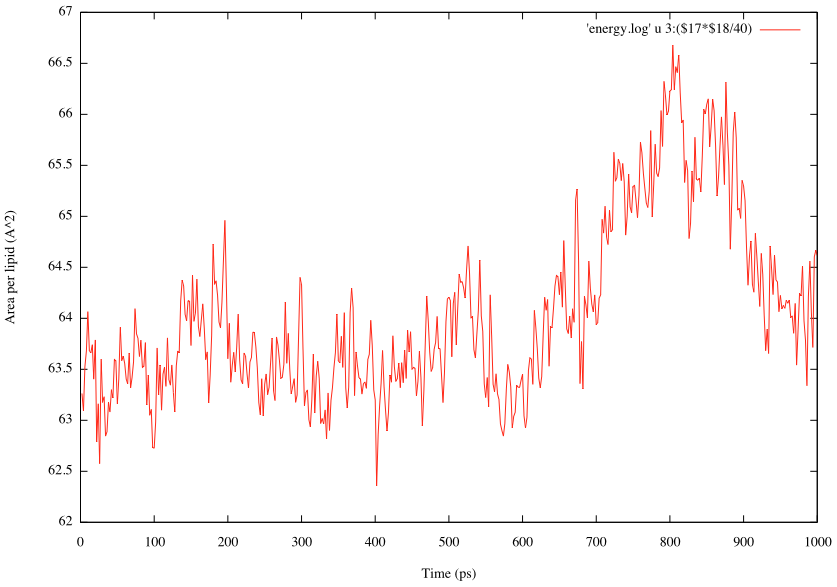
If your plot is different from our results, it may be due to different random number used in the simulations.
Although the calculated area per lipid is slightly smaller than the experimental value (Aexp = 68.3Å2 for POPC), GENESIS reproduces the averaged area per lipid of 64.7Å2 reported in the CHARMM C36 paper (J. Klauda et al., 2010 ). Longer MD simulation (~100 ns) is needed to obtain reliable structural data of lipid bilayers.
Written by Takaharu Mori@RIKEN Theoretical molecular science laboratory
June 30, 2016