3.2 String method
Files for this tutorial (tutorial-3.2.tgz)
Contents
- 3.2.3 Generate an initial pathway (Steered/Targeted MD)
- 3.2.4 Prepare inputs for string method (rpath_generator)
- 3.2.5 Equilibration along the initial pathway
- 3.2.6 String method
- 3.2.7 Visualization of pathways
- 3.2.8 Equilibration along the minimum free energy path
- 3.2.9 Replica-exchange umbrella sampling (REUS)
- 3.2.10 Analysis of free energy profile along the pathway
GENESIS 1.1.4 or later is required for this tutorial.
It is often the case that a pair of experimentally determined structures are available for a single protein, and they are different from each other due to different experimental/biochemical conditions (such as ligand-free, ligand-bound conditions). Since these structures are often related to a functionally important conformational transition (such as a transition from in-active to active state), the physical mechanism of such a transition attracts the interest of researchers. To investigate conformational transitions, molecular dynamics simulation would be suitable since simulation provides us atomistic information of dynamical process. However, unfortunately, the time-scale accessible by brute-force simulations is usually limited to several microseconds, which is too short to observe the conformational changes. The string method, introduced in this tutorial, is a powerful approach to overcome this time-scale problem. The method efficiently searches the physically most probable pathway connecting two structures, and enables us to characterize the mechanism of the conformational change.
Currently, there are three major algorithms in the string method; (i) the string method with mean forces , (ii) on-the-fly string mehtod , and (iii) the string method with swarms-of-trajectories . GENESIS supports (i) the string method with mean forces.
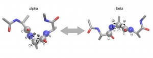
In this tutorial, we investigate the conformational change of a small peptide (alanine tripeptide). This peptide undergoes a conformational change from alpha-helix state to beta-sheet state (beta/C7eq state). Since this conformational change is well characterized by two dihedral angles, phi and psi, we will search the most probable pathway (called the minimum free energy path) in this subspace spanned by phi and psi (these are called collective variables in the context of the string method). Please note that it may take around half a whole day or longer to finish all simulations in this tutorial with a single-node machine. We recommend to use multiple computation nodes. GPU cluster is the best choice.
Unpacking the tar file creates mulptile directories in tutorial-3.2/. The initial PDB structure (solvated alanine tripeptide box) for simulation is 1_setup/wbox.pdb. The system is same as that of 2.1 REMD tutorial. So, we do not explain the system setup again. Also, the energy minimization and equilibration process is the same as “2.1.2 Minimization and pre-equilibration” in 2.1 REMD tutorial. We skip this step too and start from step 3.
3.2.3 Generate an initial pathway (Steered/Targeted MD)
We first generate data of atomistic coordinates which connects the initial (alpha-helix) and final (beta-sheet) structures. To do this, we use a steered MD simulation (also called as a Targeted MD simulation in a different context). This simulations artificially pulls the initial structure toward the final structure by imposing a restraint on the RMSD (Root Metn Squared Deviation) variable. In this case, we start from the alpha-helix structre and pull the structure toward the beta-sheet structure.
It is noted that, in the case of alanine-tripeptide, the result of steered MD is very sensitive to the random seed, compiler, hardware, etc.. so it is very hard to repduce the result below (due to subtle fluctuations of atoms, periodicity in the torsion space, low free energy barriers, and so on). Please do not run the calculation by yourself here. Please just look through the input and use the outputs already included in the directory in the next step.
The following command executes the simulation:
$ cd 3_targeted_md/
$ mpirun -np 8 spdyn run.inp
The content of run.inp is shown below. Important keywords=values are indicated by red. In the steered MD, reffile is required to give the structural information of the target state to GENESIS. In our case, we specify reffile=../1_setup/end.pdb which includes the structure of the beta state. The steered MD is turned on by steered_MD=YES. initial_rmsd is the initial RMSD value for restraint (usually RMSD value of the inital structure from the target is specified). final_rmsd is should be close to zero (excact zero might cause crash in some cases). For the calculation of RMSD, fitting of strucutre (to reffile) is needed to remove the contributios from global translation and rotations. Thus, fitting_method=TR+ROT (which means removing TRanslation and ROTation) is specified here.
[INPUT]
topfile = ../1_setup/top_all36_prot.rtf # topology file
parfile = ../1_setup/par_all36_prot.prm # parameter file
strfile = ../1_setup/toppar_water_ions.str # stream file
psffile = ../1_setup/wbox.psf # protein structure file
pdbfile = ../1_setup/start.pdb # PDB file
reffile = ../1_setup/end.pdb # PDB file for restraints
rstfile = ../2_minimize_pre-equi/step2.3.rst # restart file

[OUTPUT]
rstfile = run.rst
dcdfile = run.dcd
dcdvelfile = run.dvl

[ENERGY]
forcefield = CHARMM # CHARMM force field
electrostatic = PME # Particle Mesh Ewald method
switchdist = 10.0 # switch distance
cutoffdist = 12.0 # cutoff distance
pairlistdist = 13.5 # pair-list distance
vdw_force_switch = YES # force switch option for van der Waals
pme_nspline = 4 # order of B-spline in [PME]
pme_max_spacing = 1.0 # max grid spacing

[DYNAMICS]
integrator = LEAP # leapfrog Verlet integrator
nsteps = 500 # number of MD steps
timestep = 0.002 # timestep (ps)
eneout_period = 2 # energy output period
crdout_period = 2 # coordinates output period
velout_period = 2
rstout_period = 500 # restart output period
nbupdate_period = 2 # nonbond update period
steered_md = YES
initial_rmsd = 3.0 # initial rmsd from reffiel
final_rmsd = 0.01 # final rmsd from reffile
iseed = 1228373

[CONSTRAINTS]
rigid_bond = YES # constraints all bonds involving hydrogen

[ENSEMBLE]
ensemble = NPT # NPT ensemble
tpcontrol = LANGEVIN # thermostat and barostat
temperature = 300.00 # initial and target temperature (K)
pressure = 1.0 # initial and target pressure (atm)
isotropy = ISO # isotropic pressure coupling

[BOUNDARY]
type = PBC # periodic boundary condition

[SELECTION]
group1 = rno:1-3 and heavy

[RESTRAINTS]
nfunctions = 1
function1 = RMSD
reference1 = 3.0
constant1 = 1000.0
select_index1 = 1

[FITTING]
fitting_method = TR+ROT
fitting_atom = 1 # same group as that of restraints
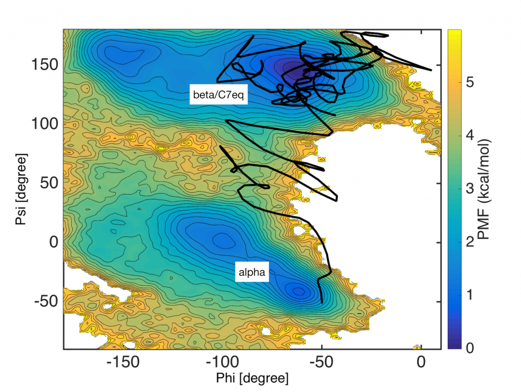
In the figure below, the trajectory of the steered MD (black line) is plotted in the collective variable space (phi and psi). The free energy surface, evaluated form very long brute-force simulations, is drawn for the reference. Although the trajectory successfully starts from the inital (alpha) to the final target (beta), there are large fluctuations in the trajecotry.
3.2.4 Prepare inputs for string method (rpath_generator)
In this step, we generate input files for string method from the result of the steered MD simulation. To do this, we use rpath_generator tool included in the GENESIS package. In the string method, we first represent a pathway of the conformational change by discretized points (called images in the context of string method) in the collective variable space (phi and psi). Then, atomistic simulation is perfomed around each image to find lower free energy regions and images are repeatedly updated to coverge to the minimum free energy path. rpath_generator provides us with the coordinates of images and restart files for atomistic simulations by analyzing the result of steered MD simulation.
rpath_generator works as follows: It first reads the steered MD trajectory projected into the collective variable space. Then, by perfoming a clustering of trajectory snapshots, it defines the coordinates of images (images are located in equal-distant manner between adjacent images). In the second step, it reads the all-atom trajectory of the steerd MD. Then, it extracts the atomistic snapshots each of which has the collective variables closest to the defined image. Finally, rpath_generator ouptuts restart files each of which contains the coordinates of both all-atoms and the corresponding image coordinates are embedded.
The following command execute rpath_generator. trj_analysis is called to produce the trajectory projected onto the phi psi space.
$ cd 4_rpath_generator/
$ trj_analysis trj_analysis.inp
$ rpath_generator rpath_generator.inp
The content of rpath_generator.inp is shown below. cvfile is a trajectory file projected on the collective variable space (generated by trj_analysis). dcdfile and dcdvelfile are trajectory files of coordinates and velocities of the steered MD, respectively. Note that generating a velocity file in steered MD is recommended since it allows rpath_generator to generate better restart files for restarting simulation. nreplica=16 specifies the number of images. Curly brackets {} in [OUTPUT] section are replaced with image indices 1,…,16. iseed is used for embedding different seeds for restart files. iter_reparam is kind of a smooting parameter for defining image coordinates (iter_reparam=10 is recommended).
By runnning this input, rpath_generator generates 16 restart files (1.rst, …, 16.rst) and 16 pdb files (1.pdb, …, 16.pdb). Restart file contains atomistic coordinates and also the coordinates of corresponding image are embedded. PDB files contain only atomistic coordinates (no information on images).
[INPUT]
cvfile = tmd.tor
pdbfile = ../1_setup/start.pdb
dcdfile = ../3_targeted_md/run.dcd
dcdvelfile = ../3_targeted_md/run.dvl

[OUTPUT]
rstfile = {}.rst
pdbfile = {}.pdb

[RPATH]
nreplica = 16
iseed = 8283
iter_reparam = 10
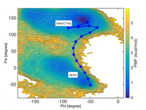
In the figure below, the images (blue circles) defined by rpath_generator are depicted in the collective variable space (phi and psi). You can see that the images are located in equi-distant manner in this 2D space.
3.2.5 Equilibration along the initial pathway
In this step, we equilibrate/relax the all-atom structures around the images for the subsequent string method calculation. We perform a simulation of 16 replicas (corresponding 16 images). The collective variables (phi and psi) of each replica is imposed by restarints whose reference values are specified by the image coordinates.
$ cd 5_equilibration/
$ mpirun -np 16 spdyn run.inp
The content of run.inp is shown below. nreplica=16 in [RPATH] means the we performs a simulation of 16 replicas. rpath_period=0 means that references of restraints (image coordinates) do not move during the simulation. Force constants for the restraints are specified by constants[12] in [RESTRAINTS]. The first value specifies the force constant of the 1st replica (image), and the 2nd value is the 2nd replica, and so on. Note that we are using a rather strong force constant (constant[12]=100.0 kcal/mol/rad2) here because strong force constants are recommended for the subsequent string method calculation. Reference values for the restraints are specified by reference[12]. We just specifies reference[12]=0.0 here because GENESIS automatically replace these values with the coordinates of images embedded in the restart files (generaged by rpath_generator). GENESIS notifies that these are replaced in the log message.
[INPUT]
topfile = ../1_setup/top_all36_prot.rtf # topology file
parfile = ../1_setup/par_all36_prot.prm # parameter file
strfile = ../1_setup/toppar_water_ions.str # stream file
psffile = ../1_setup/wbox.psf # protein structure file
pdbfile = ../1_setup/wbox.pdb # PDB file
rstfile = ../4_rpath_generator/{}.rst # restart file

[OUTPUT]
logfile = {}.log
dcdfile = {}.dcd
rstfile = {}.rst
rpathfile = {}.rpath

[RPATH]
nreplica = 16
rpath_period = 0
rest_function = 1 2

[ENERGY]
forcefield = CHARMM # CHARMM force field
electrostatic = PME # Particle Mesh Ewald method
switchdist = 10.0 # switch distance
cutoffdist = 12.0 # cutoff distance
pairlistdist = 13.5 # pair-list distance
vdw_force_switch = YES # force switch option for van der Waals
pme_nspline = 4 # order of B-spline in [PME]
pme_max_spacing = 1.0 # max grid spacing

[DYNAMICS]
integrator = LEAP
nsteps = 10000
timestep = 0.002
eneout_period = 1000
crdout_period = 1000
rstout_period = 10000
nbupdate_period = 10

[CONSTRAINTS]
rigid_bond = YES

[ENSEMBLE]
ensemble = NPT
tpcontrol = LANGEVIN
temperature = 300.0
pressure = 1.0
isotropy = ISO # isotropic pressure coupling

[BOUNDARY]
type = PBC

[SELECTION]
group1 = atomindex:15
group2 = atomindex:17
group3 = atomindex:19
group4 = atomindex:25
group5 = atomindex:27

[RESTRAINTS]
nfunctions = 2

function1 = DIHED
constant1 = 100.0 100.0 100.0 100.0 100.0 100.0 100.0 100.0 \
 100.0 100.0 100.0 100.0 100.0 100.0 100.0 100.0
reference1 = 0.0 0.0 0.0 0.0 0.0 0.0 0.0 0.0 \
 0.0 0.0 0.0 0.0 0.0 0.0 0.0 0.0
select_index1 = 1 2 3 4 # PHI

function2 = DIHED
constant2 = 100.0 100.0 100.0 100.0 100.0 100.0 100.0 100.0 \
 100.0 100.0 100.0 100.0 100.0 100.0 100.0 100.0
reference2 = 0.0 0.0 0.0 0.0 0.0 0.0 0.0 0.0 \
 0.0 0.0 0.0 0.0 0.0 0.0 0.0 0.0
select_index2 = 2 3 4 5 # PSI
3.2.6 String method
Now we perform the string method.
$ cd 6_string_method/
$ mpirun -np 16 spdyn run.inp
The content of run.inp is shown below. rpath_period in the [RPATH] specifies the step of time window during which the mean force is evaluated (by time-averaging). In this case, for every rpath_period=500 steps (corresponding to 1 ps), the image coordinates are updated according to the estimated mean forces. Typically 500-5000 steps are recommended for moderate-size biomolecules. delta in [RPATH] is the size of image update. Too large delta makes structures unstable while too small delta results in slow convergence of the pathway. Again, the reference values reference[12] for the restraints (the initial coordinates of images) are automatically replaced with those embedded in the restart files. The ouput trajectory files of the image coordinates are specified by rpathfile={}.rpath in [OUTPUT].
[INPUT]
topfile = ../1_setup/top_all36_prot.rtf # topology file
parfile = ../1_setup/par_all36_prot.prm # parameter file
strfile = ../1_setup/toppar_water_ions.str # stream file
psffile = ../1_setup/wbox.psf # protein structure file
pdbfile = ../1_setup/wbox.pdb # PDB file
rstfile = ../5_equilibration/{}.rst

[OUTPUT]
logfile = {}.log
dcdfile = {}.dcd
rstfile = {}.rst
rpathfile = {}.rpath

[RPATH]
nreplica = 16
rpath_period = 500
delta = 0.2
smooth = 0.0
rest_function = 1 2

[ENERGY]
forcefield = CHARMM # CHARMM force field
electrostatic = PME # Particle Mesh Ewald method
switchdist = 10.0 # switch distance
cutoffdist = 12.0 # cutoff distance
pairlistdist = 13.5 # pair-list distance
vdw_force_switch = YES # force switch option for van der Waals
pme_nspline = 4 # order of B-spline in [PME]
pme_max_spacing = 1.0 # max grid spacing

[DYNAMICS]
integrator = LEAP
nsteps = 50000
timestep = 0.002
eneout_period = 500
crdout_period = 500
rstout_period = 500
nbupdate_period = 10

[CONSTRAINTS]
rigid_bond = YES

[ENSEMBLE]
ensemble = NPT
tpcontrol = LANGEVIN
temperature = 300.0
pressure = 1.0
isotropy = ISO # isotropic pressure coupling

[BOUNDARY]
type = PBC

[SELECTION]
group1 = atomindex:15
group2 = atomindex:17
group3 = atomindex:19
group4 = atomindex:25
group5 = atomindex:27

[RESTRAINTS]
nfunctions = 2

function1 = DIHED
constant1 = 100.0 100.0 100.0 100.0 100.0 100.0 100.0 100.0 \
 100.0 100.0 100.0 100.0 100.0 100.0 100.0 100.0
reference1 = 0.0 0.0 0.0 0.0 0.0 0.0 0.0 0.0 \
 0.0 0.0 0.0 0.0 0.0 0.0 0.0 0.0
select_index1 = 1 2 3 4 # PHI

function2 = DIHED
constant2 = 100.0 100.0 100.0 100.0 100.0 100.0 100.0 100.0 \
 100.0 100.0 100.0 100.0 100.0 100.0 100.0 100.0
reference2 = 0.0 0.0 0.0 0.0 0.0 0.0 0.0 0.0 \
 0.0 0.0 0.0 0.0 0.0 0.0 0.0 0.0
select_index2 = 2 3 4 5 # PSI
3.2.7 Visualization of pathways
The trajectory of image coordinates is written in 6_string_method/{}.rpath files. By using these coordintes, the evolution of the pathway can be visualized with a python script.
$ cd 7_visualize/
$ python plot.py
# unix
$ dipaly plot.png
# mac
$ open plot.png
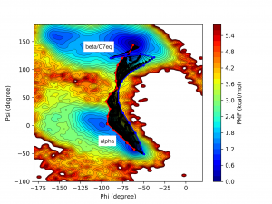
In the figure below, the initial pathway is plotted by the blue line. The black lines represent intermediate pathways during the string method calculation. The red line is the final converged pathway (supposed to be the minimum free energy path).
3.2.8 Equilibration along the minimum free energy path
Now we have the minimum free energy path connecting alpha-helix and beta-sheet. In the following, we are going to characterize the pathway in terms of energetics; free energy profile along the pathway. In order to evaluate the free energy profile, more samplings are needed for good statistics. To do this, at first, we will equilibrate the system using a weak force constant of 5.0 kcal/mol/rad2 (for sufficient phase space overlaps required by subsequent reweighting analysis, such as MBAR or WHAM).
$ cd 8_equilibration/
$ mpirun -np 16 spdyn run.inp
The content of run.inp is shown below. Again, the reference values reference[12] for the restraints (the coordinates of images) are automatically replaced with those embedded in the restart files (in this case, those of the last snapshots in the string method calculation)
[INPUT]
topfile = ../1_setup/top_all36_prot.rtf # topology file
parfile = ../1_setup/par_all36_prot.prm # parameter file
strfile = ../1_setup/toppar_water_ions.str # stream file
psffile = ../1_setup/wbox.psf # protein structure file
pdbfile = ../1_setup/wbox.pdb # PDB file
rstfile = ../6_string_method/{}.rst

[OUTPUT]
logfile = {}.log
dcdfile = {}.dcd
rstfile = {}.rst
rpathfile = {}.rpath

[RPATH]
nreplica = 16
rpath_period = 0
rest_function = 1 2

[ENERGY]
forcefield = CHARMM # CHARMM force field
electrostatic = PME # Particle Mesh Ewald method
switchdist = 10.0 # switch distance
cutoffdist = 12.0 # cutoff distance
pairlistdist = 13.5 # pair-list distance
vdw_force_switch = YES # force switch option for van der Waals
pme_nspline = 4 # order of B-spline in [PME]
pme_max_spacing = 1.0 # max grid spacing

[DYNAMICS]
integrator = LEAP
nsteps = 5000
timestep = 0.002
eneout_period = 1000
crdout_period = 1000
rstout_period = 5000
nbupdate_period = 10

[CONSTRAINTS]
rigid_bond = YES

[ENSEMBLE]
ensemble = NPT
tpcontrol = LANGEVIN
temperature = 300.0
pressure = 1.0
isotropy = ISO # isotropic pressure coupling

[BOUNDARY]
type = PBC

[SELECTION]
group1 = atomindex:15
group2 = atomindex:17
group3 = atomindex:19
group4 = atomindex:25
group5 = atomindex:27

[RESTRAINTS]
nfunctions = 2

function1 = DIHED
constant1 = 5.0 5.0 5.0 5.0 5.0 5.0 5.0 5.0 \
 5.0 5.0 5.0 5.0 5.0 5.0 5.0 5.0
reference1 = 0.0 0.0 0.0 0.0 0.0 0.0 0.0 0.0 \
 0.0 0.0 0.0 0.0 0.0 0.0 0.0 0.0
select_index1 = 1 2 3 4 # PHI

function2 = DIHED
constant2 = 5.0 5.0 5.0 5.0 5.0 5.0 5.0 5.0 \
 5.0 5.0 5.0 5.0 5.0 5.0 5.0 5.0
reference2 = 0.0 0.0 0.0 0.0 0.0 0.0 0.0 0.0 \
 0.0 0.0 0.0 0.0 0.0 0.0 0.0 0.0
select_index2 = 2 3 4 5 # PSI
3.2.9 Replica-exchange umbrella sampling (REUS)
Next, we generate samples along the minimum free energy pathway. Although umbrella sampling is usually used for this purpose, this tutorial uses REUS since it is more powerful and easily available in GENESIS. For details of REUS in GENESIS, please see 2.2 REUS tutorial.
$ cd 9_reus/
$ mpirun -np 16 spdyn run.inp
The content of run.inp is shown below. Again, the reference values reference[12] for the restraints (the coordinates of images) are automatically replaced with those embedded in the restart files.
[INPUT]
topfile = ../1_setup/top_all36_prot.rtf # topology file
parfile = ../1_setup/par_all36_prot.prm # parameter file
strfile = ../1_setup/toppar_water_ions.str # stream file
psffile = ../1_setup/wbox.psf # protein structure file
pdbfile = ../1_setup/wbox.pdb # PDB file
rstfile = ../8_equilibration/{}.rst

[OUTPUT]
logfile = {}.log
dcdfile = {}.dcd
rstfile = {}.rst
remfile = {}.rem # parameter index file

[REMD]
dimension = 1
exchange_period = 1000
type1 = RESTRAINT
nreplica1 = 16
cyclic_params1 = NO
rest_function1 = 1 2

[ENERGY]
forcefield = CHARMM # CHARMM force field
electrostatic = PME # Particle Mesh Ewald method
switchdist = 10.0 # switch distance
cutoffdist = 12.0 # cutoff distance
pairlistdist = 13.5 # pair-list distance
vdw_force_switch = YES # force switch option for van der Waals
pme_nspline = 4 # order of B-spline in [PME]
pme_max_spacing = 1.0 # max grid spacing

[DYNAMICS]
integrator = LEAP
nsteps = 100000
timestep = 0.002
eneout_period = 100
crdout_period = 100
rstout_period = 1000
nbupdate_period = 10

[CONSTRAINTS]
rigid_bond = YES

[ENSEMBLE]
ensemble = NPT
tpcontrol = LANGEVIN
temperature = 300.0
pressure = 1.0
isotropy = ISO # isotropic pressure coupling

[BOUNDARY]
type = PBC

[SELECTION]
group1 = atomindex:15
group2 = atomindex:17
group3 = atomindex:19
group4 = atomindex:25
group5 = atomindex:27

[RESTRAINTS]
nfunctions = 2

function1 = DIHED
constant1 = 5.0 5.0 5.0 5.0 5.0 5.0 5.0 5.0 \
 5.0 5.0 5.0 5.0 5.0 5.0 5.0 5.0
reference1 = 0.0 0.0 0.0 0.0 0.0 0.0 0.0 0.0 \
 0.0 0.0 0.0 0.0 0.0 0.0 0.0 0.0
select_index1 = 1 2 3 4 # PHI

function2 = DIHED
constant2 = 5.0 5.0 5.0 5.0 5.0 5.0 5.0 5.0 \
 5.0 5.0 5.0 5.0 5.0 5.0 5.0 5.0
reference2 = 0.0 0.0 0.0 0.0 0.0 0.0 0.0 0.0 \
 0.0 0.0 0.0 0.0 0.0 0.0 0.0 0.0
select_index2 = 2 3 4 5 # PSI
3.2.10 Analysis of free energy profile along the pathway
Finally, we analyze the output of REUS and evaluate the free energy profile along the converged pathway. A shell script for this analysis is 10_analysis/run.sh. In the script, several analysis tools of GENESIS are called.
$ cd 10_analysis/
$ ./run.sh
$ python plot.py
# unis
$ display plot.png
# mac
$ open plot.png
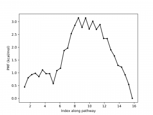
After running the script, we get pmf.dat whose 1st column contains image index and 2nd column is the free energy profile. The result should like below.
Details of the analysis is beyond the scope of this tutorial. Usage of the analysis tools of GENESIS will be explained in “Tutorials of trajectory analysis“. Here, we just summarize the analysis steps performed by the script (run.sh):
- calls remd_convert to convert replica-trajectories to sorted parameter-trajectories (i.e., trajectories with the same reference values)
- calls trj_analysis to calculate dihedral angles from parameter-trajectories
- calls mbar_analysis to perform MBAR and obtain unbiasing weights from dihedral angle data
- calls pathcv_analysis to get tangential and perpendicular coordinates to the pathway
- calls pmf_analysis to evaluate free energy profile (pmf.dat) from the MBAR weights and tangential coordinates to the pathway
Written by Yasuhiro Matsunaga@RIKEN Computational biophysics research team
Created August 26, 2016
Updated May 1, 2017